| |
Applies To |
|
|
| |
Product(s): |
WaterCAD, WaterGEMS |
|
| |
Version(s): |
CONNECT Edition, V8i |
|
| |
Area: |
Layout and Data Input |
|
Overview
The Pressure Dependent Demands (PDD) feature enables you to perform a hydraulic simulation in which the nodal demands can vary based on changes in nodal pressure. This article explains how to set up a PDD simulation in WaterCAD and WaterGEMS and also provides suggestions for PDD input data.
Note: demands are always treated as pressure dependent during a transient simulation in HAMMER. See more here.
Background
Some types of water demands are volume-based, in that the demand is independent of available pressure. Examples of volume-based demand sources are washing machines, dishwashers, and toilets (the same volume is used regardless of the pressure). Other demands are pressure-dependent, meaning water usage decreases with a decrease in pressure. Pressure-based demand examples include showers, sprinklers, and leaks.
Typically, water modeling programs assume that all demands are volume-based, and maintain the user-input demand regardless of the calculated available pressure. Although this assumption works well under the normal range of pressure conditions, it loses accuracy if an episode such as a fire or pump outage causes a significant decrease in system pressure.
One option for modeling demands that vary based on pressure is to set up model nodes as simple flow emitters, using the emitter coefficient property of the node. Because the flow emitter approach places no upper limit on the amount of water demanded with increasing pressure, it is most useful for determining water consumption by a free-discharge element such as a sprinkler or broken pipe. However, other pressure-based demand types result in no additional consumption once the pressure is above a certain threshold value, such that use of flow emitters in the model could skew water consumption to be unrealistically high in higher-pressure areas. Another limitation of flow emitters is that they will result in calculation of a negative demand, or inflow, when the pressure is negative.
WaterCAD and WaterGEMS have a Pressure Dependent Demands (PDD) feature that allows for more control over demand calculation. In many instances where pressure affects water use, the PDD feature will provide a more realistic result than simply placing flow emitters on nodes.
Using PDD, you can:
- Analyze pressure-dependent demands at a single node, subset of nodes, or all nodes
- Define the reference pressure at which 100 percent of the specified reference demand can be met
- Define the threshold pressure beyond which an increase in pressure results in no additional demand increase
- Combine PDD and volume-based demands at individual nodes
- Determine the actual supplied demand at a PDD node, as well as the demand shortfall (see the "Demand Shortage" result field)
- Obtain a result of zero for pressure-dependent demands when the pressure is less than or equal to zero
- Present the calculated PDD and the associated results in a table and graph
WaterGEMS and WaterCAD use a formulation we call the Modified Global Gradient Algorithm. Instead of single formulation to solve PDD, WaterGEMS and WaterCAD have two methods that are both flexible in themselves:
1. Q = a P^n where n is a variable
2. Piecewise linear curve with any monotonically increasing function
The information below discussing setting up and using PDD in a water model.
Setting Up the PDD Function
- Open the Pressure Dependent Demand menu item
- Click the New button to create a new PDD function
- The Function Type can either be Power Function or Piece-wise Linear
- The Power Function option is used to define the exponential relationship between the nodal pressure and demand. The ratio of actual supplied demand to the reference demand (i.e., percentage of defined nodal demand designated as pressure-dependent) is defined as a power function of the ratio of actual pressure to reference pressure. (Defining of reference pressure and pressure-dependent demand percentage is done in the Alternative, as described in the next section.) Using a power equation for your Pressure Dependent Demands is like you are assuming that each 'demand' in your system acts like an orifice. The orifice equation can be written like this: Q = K*P0.5 Where Q is flow through the orifice, P is pressure upstream of the orifice, and K is some coefficient (which is a function of orifice area, coefficient of discharge, etc.) You can specify a desired Power Function Exponent. The default value provided is 0.5, which is the exponent used in the orifice equation. By checking the box for "Has Threshold Pressure?" you can define a pressure value that maximizes the computed pressure-dependent demand (i.e., demand remains constant when the pressure exceeds the threshold value). If you do not define a threshold pressure, demand will increase with pressure regardless of how high it is. Since many PDD simulations are focused on the effects of lower pressure conditions, it is often not necessary to define a threshold pressure.
See the screenshot below for Power Function:

Example: If pressure on J-10 is 40% of the Pressure (Reference) set in the Pressure Dependent Demand Alternative (explained below), then going by the graph above (or by computing 0.400.5), the demand on that given junction will be 63.2% of what was set initially. In other words, if J-10 had a demand of 100gpm, and the Pressure (Reference) is set to 150psi, then if pressure on J-10 drops to 60psi (which is 40% of the 150psi), the demand will not be 100gpm any more--it will be 63.2 gpm. The Piece-wise Function allows you to manually specify the relationship between reference pressure and demand, as shown in the screenshot below:

Example: If pressure on J-10 is 65% of the Pressure (Reference) set in the Pressure Dependent Demand Alternative (explained below), then going by the table above, the demand on that given junction will be 80% of what was set initially. In other words, if J-10 had a demand of 200 gpm, and the Pressure (Reference) is set to 200psi, then if pressure on J-10 drops to 130psi (which is 65% of the 200psi), the demand will not be 200 gpm anymore, it will be 160 gpm (80%).
Note: If you are using a piece-wise linear function make sure the changes aren't too abrupt on the curve, otherwise the solver may have a more difficult time arriving at a solution. If you have too abrupt a change you may get a "network unbalanced" user notification. To resolve this you could try to gradually decrease the demand.
Create a Scenario that Assigns a PDD Function to an Alternative
This section describes how to create and configure a new Scenario and Alternative to run your PDD analysis.
-
- Go to Analysis > Scenarios. Create a new Scenario.
- Double-click on the scenario you just created. Click on the drop-down menu right next to Pressure Dependent Demand. Click on New.
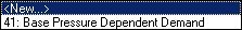
- Assign a name to the new alternative or keep the default as Pressure Dependent Demand Alternative - 1
- Go to Analysis > Alternatives. Expand the Pressure Dependant Demand alternative and double-click on the one you just created.
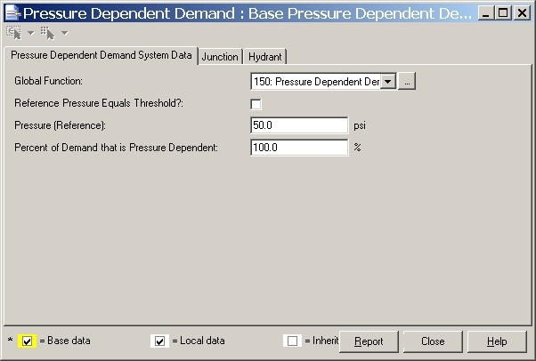
- Select the Global Function you created earlier. See screenshot below:
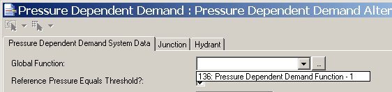
- Set the Pressure (Reference), or check the Reference Pressure Equals Threshold? box if you want it to apply.
Often, the Reference Pressure will be defined as the typical pressure at a node under typical demand conditions (corresponding to the full demand). However, if you are analyzing pressure-dependent demands for multiple nodes with significantly different typical pressures, you will need to override this system Reference Pressure on a node-by-node basis, as described in the next section.
- You can set a percentage of the demand that can be pressure dependent. For example, in that case that J-10 has a demand of 200 gpm, you can set 20% (40 gpm) that will not be affected regardless of pressure changes on that node, and the rest of the 80% (120 gpm) will comply to the Pressure Dependent Demand function. If that doesn't apply, keep Percent of Demand that is Pressure Dependent to 100%
- Click on Close.
Assigning PDD on Specific Nodes
- To override the PDD settings locally on specific junctions (for example to apply a different reference pressure in cases where each demand has different pressures that correspond to full-demand conditions), go to the Junction/Hydrant Tab on the Pressure Dependent Demand Alternative window.
- Check the box under "Use Local Pressure Dependent Demand Data?" Then, select the Local Function from the drop-down menu (you can also create a different PDD function that can be used on selected junctions).
- Check the Reference Pressure Equals Threshold? or set the Pressure (Reference), if it applies.
- You may want to set the Reference Pressures for your nodes equal to their "typical" pressures, as computed in a separate representative Scenario. One way to do this is to:
- Go to your "typical" scenario, open a junction table, sort it by ID, click the first cell in the Pressure column, hold the Shift key, and click the last cell in the column. Then, CTRL+C to copy the data to your Windows clipboard.
- Return to your PDD alternative, go to the Junction tab, and right-click and Global Edit the "Use Local Pressure Dependent Demand Data?" column to set all values to TRUE.
- Sort the junctions by ID.
- Click the Pressure (Reference) column heading to select the cells in that column, then CTRL+V to paste pressure values from your clipboard. Spot check the pressures to be sure they pasted correctly.

Set up Calculation Options
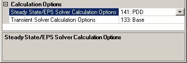
- You'll also need to set up the Calculation Option for the new scenario you created. Go to Analysis > Calculation Options.
- Click on New button. Double click on the newly created calculation option.

- Set Use Pressure Dependent Demand? to True.
- For Pressure Dependent Demand Selection you can either choose or a Selection Set (with nodes where the PDD alternative will apply to, with all the rest always using their regular demands) you created from that list.
- Now, assign this Calculation Option to the PDD scenario, by double-clicking on the scenario, then choose the PDD calculation option under the Calculation Option drop down menu.
Now you can run the scenario.
Additional Resources: Pressure Management and Repair of Pipes - for Active Leakage Control (webinar)
Viewing Results
After computing a model with PDD, you can view the following results:
- "Results" section of node properties
- Demand - this will show the calculated demand that the model used during the calculations, based on the PDD function.
- Pressure - this shows the corresponding pressure, which is compared to the reference pressure in the PDD alternative along with the PDD function, to determine the corresponding calculated demand
- "Results (Pressure Dependent Demands)" section of node properties
- Demand (Target) - this displays the base flow entered in the node's demand collection, and used as a reference point. Typically the base flow (demand target) represents the demand at full pressure, so anything lower than this (due to low pressure) would be considered below target.
- Demand Shortage - represents the difference between the target demand and the calculated demand based on the pressure at the node. The target demand is the base flow value that you enter for the node. If the pressure is lower than the reference pressure (set in the PDD alternative), the calculated demand will be lower than the target demand and you will have a positive "shortage". If the pressure is higher than the reference pressure, the calculated demand will be higher than the target demand and you will have a negative "shortage". In some cases you may set a threshold such that the demand cannot rise above the target (base flow) in which case a negative shortage will not occur. When the base flow of a demand node is considered to be the fully satisfied demand, then the "demand shortage" field can help indicate how much of a shortfall there is, if the pressure is too low. For example you could color code on this field to find areas where the demands cannot be fully supplied because the pressure is below the reference pressure.
- Demand (Cumulative) - This is a timestep-sensitive (use the Time Browser) result field that shows the total required demand volume (based on the "Demand (Target)" over time) at the current node up to the current time step. This can be used as a reference for example when viewing the last timestep of the EPS run, to understand the full volume that would be demanded under full pressure conditions.
- Supply (Cumulative) - Like above, this is a timestep sensitive result. It shows the actual calculated volume of demand up to the current time step, based on the available pressure and PDD function. It is used alongside the "Demand (Cumulative)" to understand how much can be supplied based on available pressure and compared to what would have been supplied at full pressure conditions.
- Shortfall (Cumulative) - Like above, this is a timestep sensitive result. It shows the demand shortage as a volume, based on the difference between the target demand volume and the supply (calculated) demand volume. This can be useful to capture the overall shortage over the course of an EPS, for example when viewing the last timestep.
Note that annotation and color coding can be used on these result fields. For example you could color code on the Demand Shortage field to find areas where the demands cannot be fully supplied because the pressure is below the reference pressure.
PDD vs PDA (EPANET)
Starting with EPANET version 2.2, a new PDA (pressure driven analysis) option has been made available in EPANET, similar to the PDD feature in WaterGEMS/WaterCAD.
To configure PDD in WaterGEMS/WaterCAD in the same way that PDA is implemented as of EPANET version 2.2:
- Use the Power Function PDD function type with an exponent equal to what is seen in EPANET 2.2 (default of 0.5)
- Check the box for "Has threshold pressure" and set it equal to the EPANET PDA "required pressure" value. PDA in EPANET currently assumes that the full demand is used when the pressure is above the "Required" pressure.
- In the PDD alternative, check the box for "reference pressure equals threshold pressure" and set the percent of demand that is PDD to 100%.
- In the Calculation Options, choose "<All Nodes>" for the "Pressure Dependent Demands Selection Set". PDA in EPANET currently applies to all demand nodes.
Note: this is subject to change if newer versions of EPANET introduce new capabilities or other changes to PDA. See more about PDA in the EPANET 2.2 release notes here.
See Also
Pressure dependent demands and negative pressure
Modeling intermittant or closed off demands
Article In Other Languages