| Product(s): |
OpenFlowsTM FLOODTM |
| Version(s): |
10.XX.XX.XX |
| Area: |
Modeling |
|
Overview
Sometimes we may need to impose specific time series input for pre-defined locations. This option is quite frequent when configuring atmospheric forcing in a flood model – particularly rainfall depth property.
In this section we will illustrate how to properly prepare and create a rainfall depth timeseries input file, and how to configure the model to be able to ingest it in the whole spatial domain (rainfall constant in space). OpenFlows FLOOD also allows to impose rainfall depth or intensity, any of them variable in space and time based on multiple rainfall time series instead only one in the whole domain – but we don’t describe those advanced options in this generic guide – a specific guide on this thematic will be later generated and shared in Bentley Communities.
We will exemplify this application based in the existing dataset from Graz, and then we will create a new simulation.
You can download in Bentley Communities a sample workspace with time-variable rainfall (and constant in space)
Method
Create timeseries input file (variable rainfall)
- Be sure that you have loaded the existing workspace “Graz”
- Go to Explorer window, and under the Project Tree, expand the tree till “Boundary Conditions” storage directory (under “General Data”).
- We are now ready to create a timeseries file inside “Boundary Conditions” directory. Note that you can create a time series in any directory under “General Data” folder. Select “Boundary Conditions” by left-clicking. Then right-click, and select the option “Create File” – “Time Series File…”.
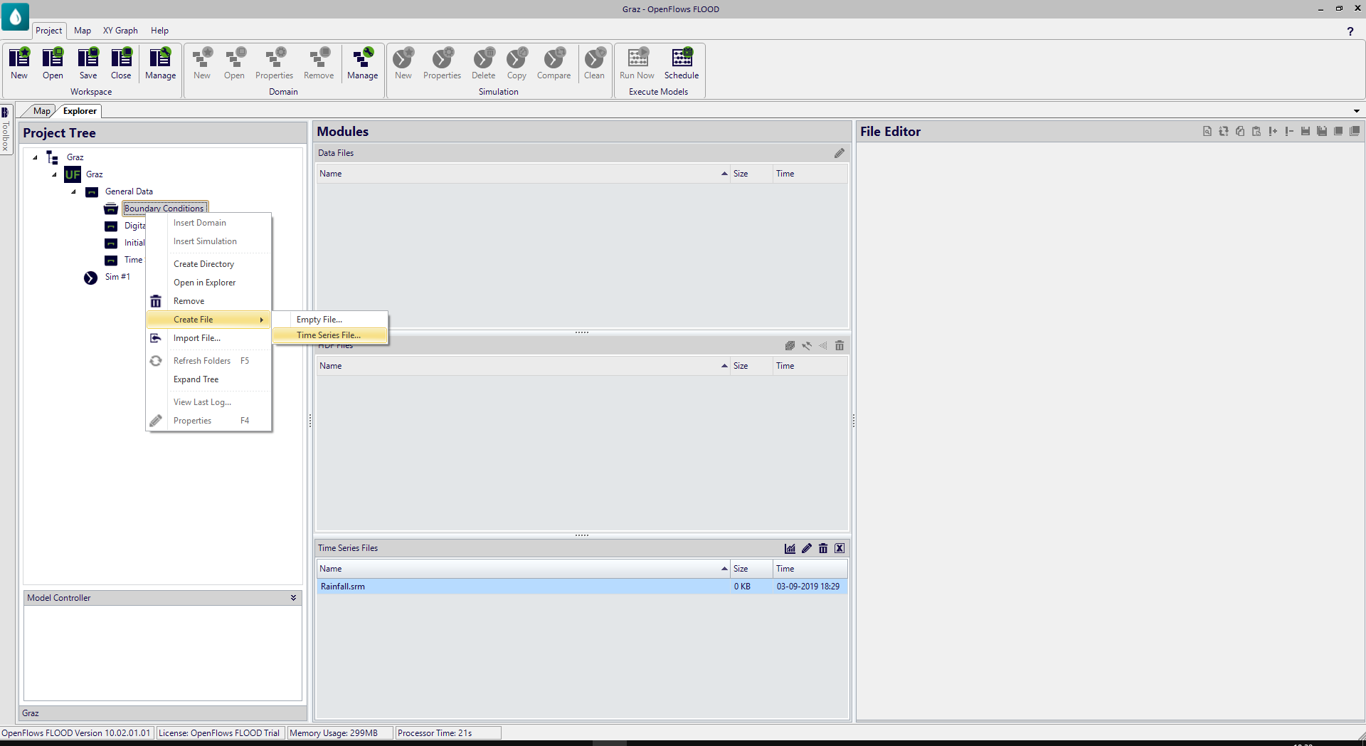
Figure 1 – Creating a new Time Series File inside OpenFlows FLOOD
- Let’s name the file “Rainfall_2.srm” (you will see that a file called “Rainfall.srm” already exists in the directory. In this exercise we are showing how to create and configure a similar file, so that’s why we are naming it “Rainfall_2.srm”. Anyway, we could name it whatever we want. We just need to be careful later when configuring the module data file, which should properly point to the desired timeseries filename and folder.
- After creating the timeseries file, you’ll be able to see it under “Time Serie Files” tab. Select (left-click) “Rainfall_2.srm” and then right-click and select “Open”:
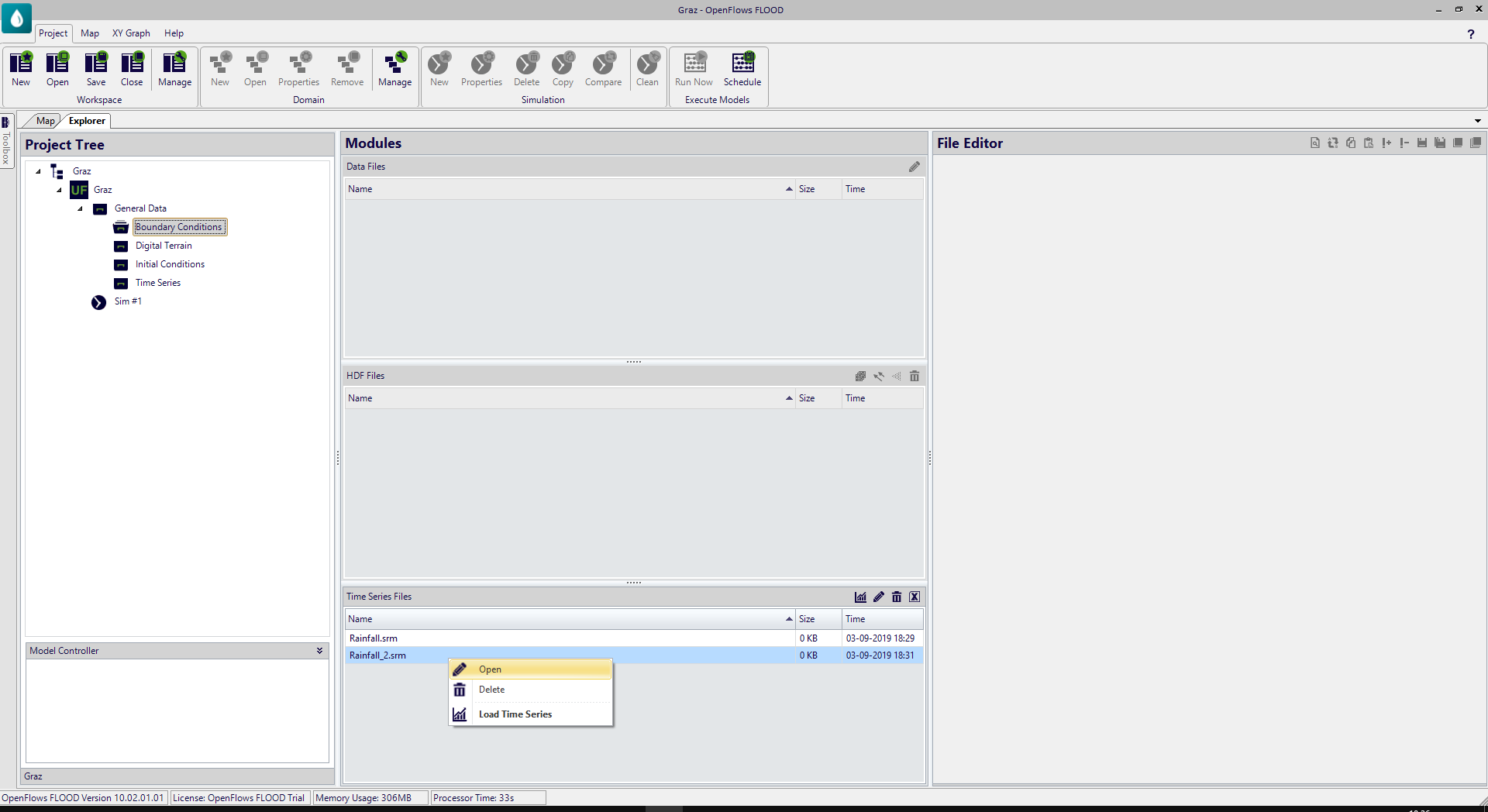
Figure 2 – Opening the created Time Series file
- The “Rainfall_2.srm” timeseries file will open for edition in the File Editor:
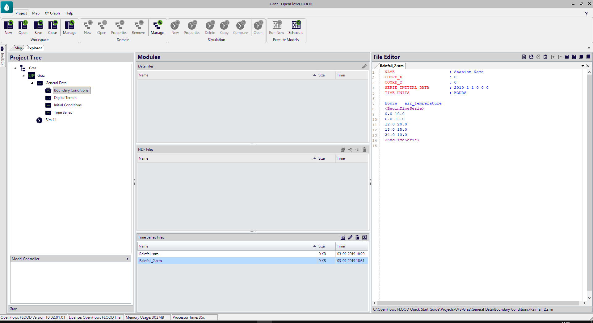
Figure 3 – Visualizing the TimeSeries file in File Editor
You will observe that the created timeseries file has 5 initial keywords, and after that, a block BeginTimeSerie/EndTimeSerie where the first column is the instant and the second is in fact an air temperature timeseries. The details about the keywords are described next:
- NAME: This is the name that will be used by the model to identify the timeseries
- COORD_X and COORD_Y: These keywords represent the spatial location, and since we are using the default configuration of spatially constant rainfall, the timeseries location is not relevant.
- SERIE_INITIAL_DATA: This is the initial timeseries instant. It should cover the whole simulation period (i.e., starting at the same time or before the simulation start time; and ending at the same time or after the simulation end time).
- TIME_UNITS: This the time unit used in the first column of the timeseries. One can use HOURS, MINUTES, SECONDS, DAYS, MONTHS, YEARS.
As regards to the contents inside the block BeginTimeSerie/EndTimeSerie, above that block you can see a line with the headers of the column names (by default the created timeseries file generates a line with “hours” and “air_temperature”) – this is not read by the model and is merely informative for the user. If we delete this line, there is no impact on the model running in any way.
Now we need to edit the file in order to represent a valid rainfall event: For now, the easiest way will be to copy the data from “rainfall.srm” timeseries file to “rainfall_2.srm” (however, the user can later insert any other data as desired) . To do so, follow the next procedure:
- Open the file “Rainfall.srm”: Select (left-click) “Rainfall.srm” and then right-click and select “Open”. Now we have two timeseries files opened for edition in OpenFlows FLOOD. This “Rainfall.srm” has two columns: the first with the hours after
- In File Editor tab, select the whole text from the “Rainfall.srm” (drag the whole text with the mouse), then press the right mouse button and select “Copy” (as an alternative, you can press Control+C, or use the button
 ):
):
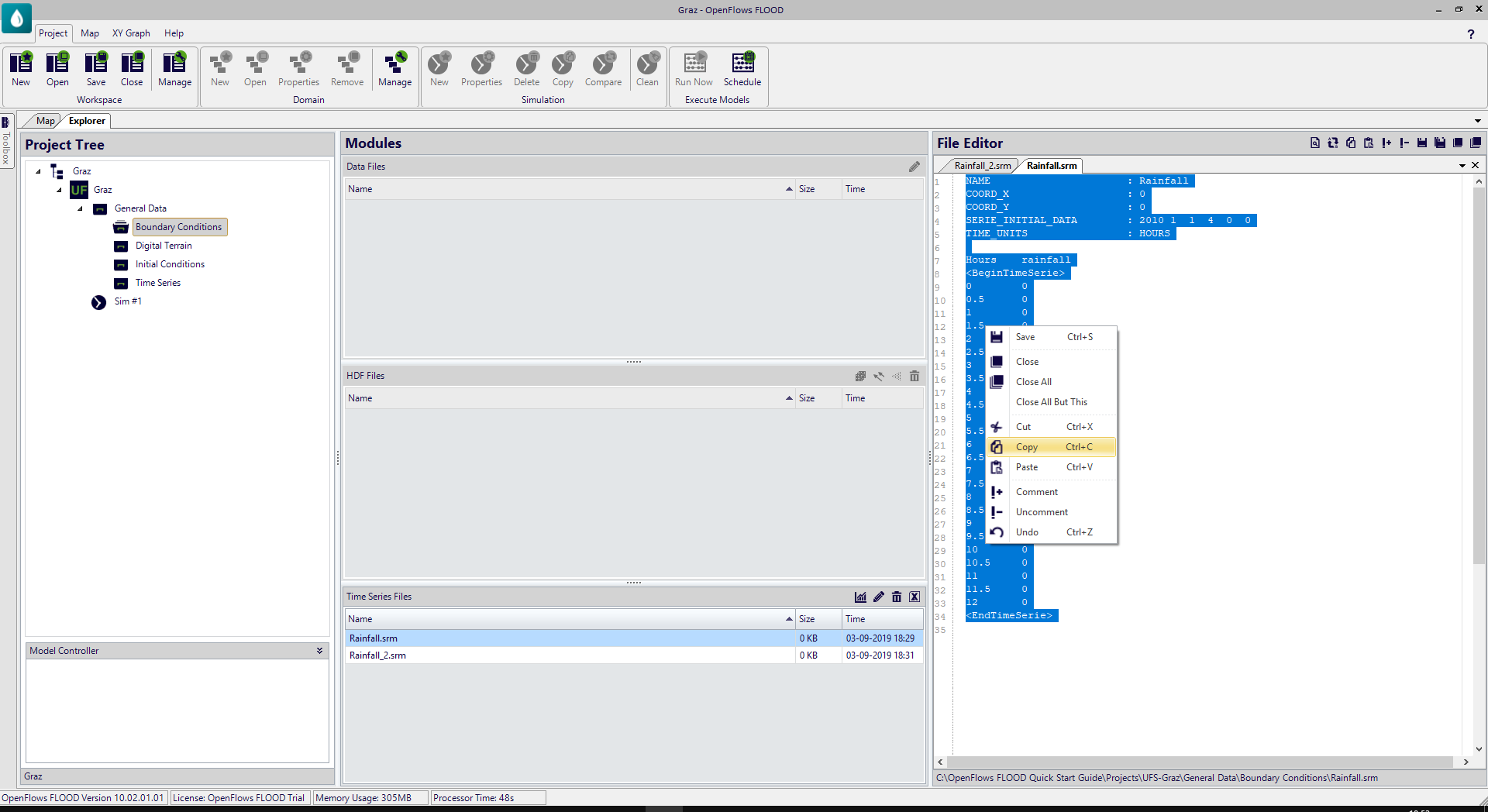
Figure 4 – Copying content from one timeseries file to another one
- In File Editor, select now the tab relative to “Rainfall_2.srm”, delete all the text, press the right mouse button and select “Paste” (as an alternative, you can press Control+V, or use the button
 ).
).
- Save the changes on “Rainfall_2.srm” file: press the right mouse button and select Save (as an alternative, you can press Control+S or click on the button
 ).
).
Now we have successfully finished the generation and configuration of a new rainfall timeseries input file. The next step is to configure the model to consume the spatially constant and timely variable rainfall depth timeseries as a boundary condition.
Configure the model to ingest the generated timeseries
We will show how to configure the model to be able to ingest the previously generated rainfall depth timeries in the whole spatial domain (rainfall constant in space). This will be illustrated with a new simulation:
- Create a new simulation (follow instructions from chapter 4.4), name it “Sim #2 – variable rainfall” and include all the default module data files + “Atmosphere” data file.
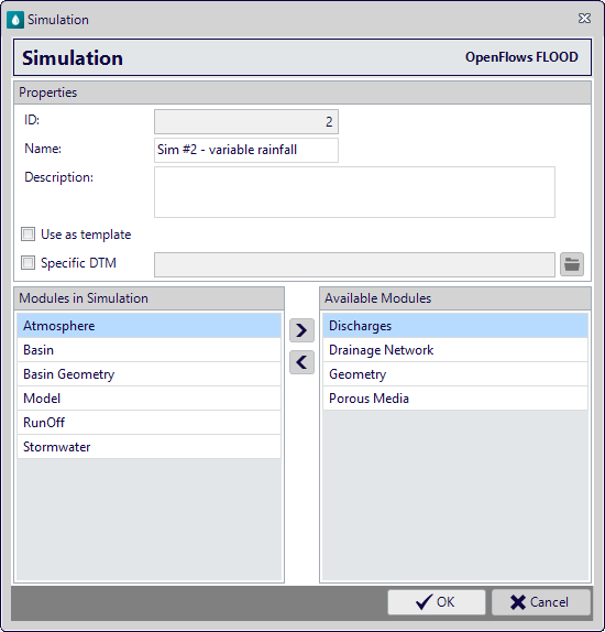
Figure 5 – Creating a new simulation
You will find that under the created simulation, 6 module data files are generated. The main difference from the other existing simulation (Sim #1) is the module data file relative to atmosphere data file (Atmosphere_2.dat):
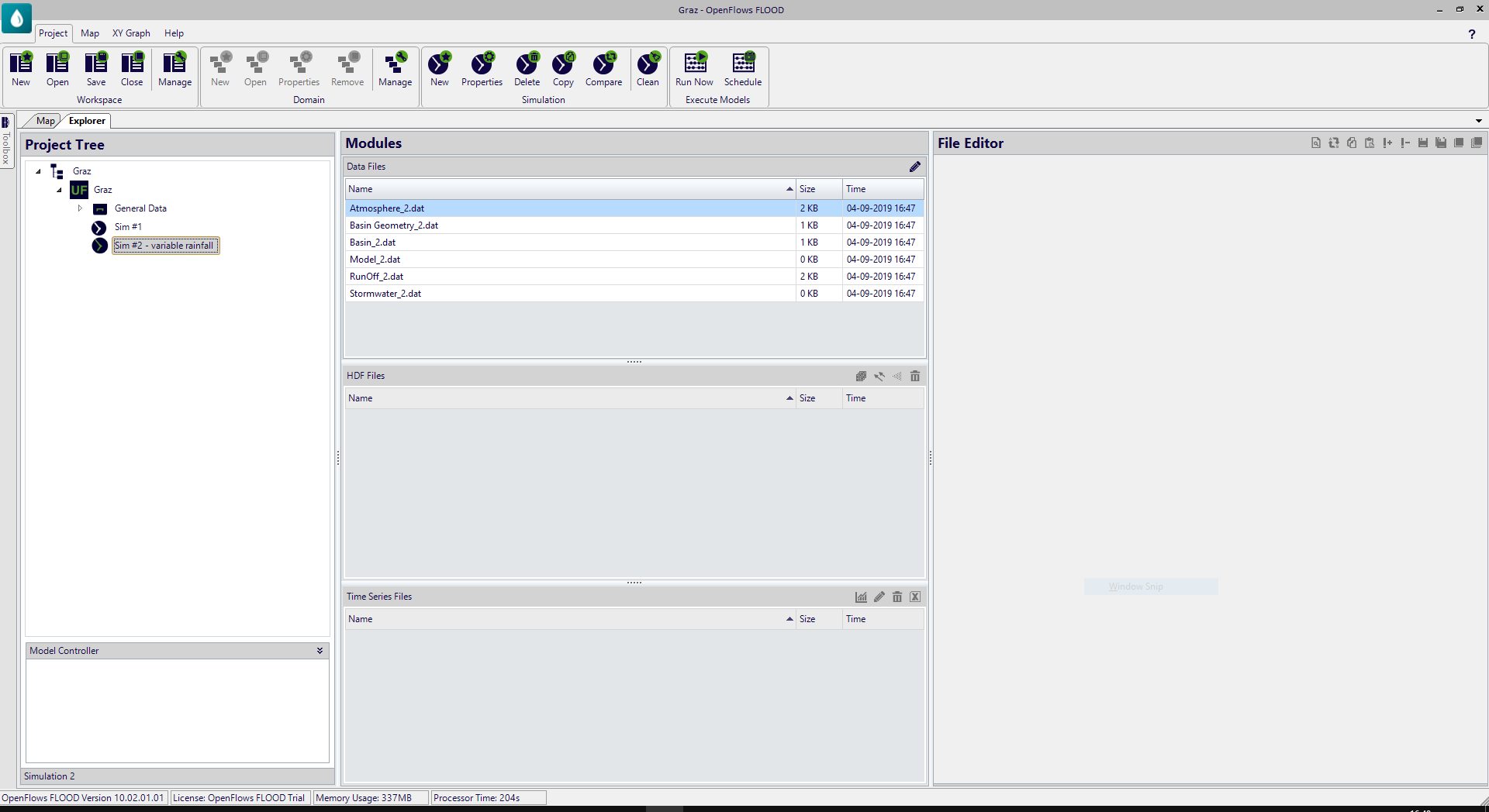
Figure 6 – Existing modules in “Sim #2 – variable rainfall”
- We want to copy the content of each module data file, from “Sim #1” to “Sim #2 – variable rainfall”. We can do it by opening the 5 pairs of files (Basin_Geometry_1.dat -> Basin_Geometry_2.dat; Basin_1.dat _> Basin_2.dat; Model_1.dat -> Model_2.dat; RunOff_1.dat -> RunOff_2.dat; and Stormwater_1.dat -> Stormwater_2.dat) using the File Editor, and then using the copy / paste clipboard or as an alternative, use the File editor buttons
 , and
, and  for saving the files.
The next step is to edit the Atmosphere module data file (Atmosphere_2.dat):
- In Project Tree, under “Sim # 2 – variable rainfall” double-click on the module data file “Atmosphere_2.dat” in order to edit it in File Editor.
Expand “precipitation” property, and ensure it is enabled. Still inside “Precipitation” property, Expand “Values”, and configure the following options:
- Impose field from file: Time Series
- Filename: (select the path pointing to the created time series file)
- Data column: 2
- Map output: select “True” if you want to output this property to the gridded outputs (HDF5) (be sure that option “Output” > “Map Output” is = “True”)
- Time Series output: select "True" in case you want to include this property in a timeseries output file (be sure that option “Output” > “Time Series” is = “True” and you have a valid “time series location” path duly defined)
The modified version of Atmosphere_2.dat is as follows:
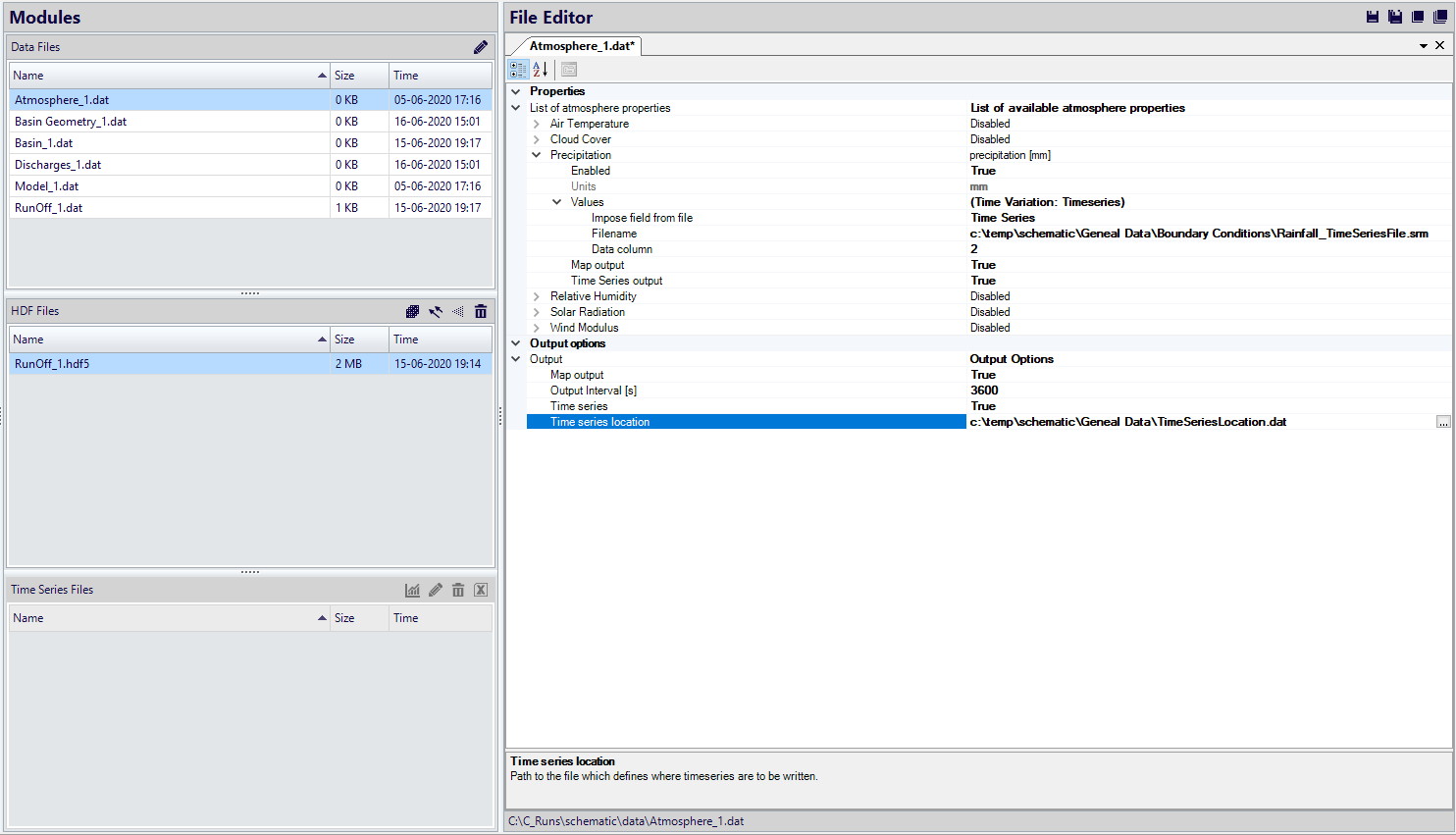
Figure 7 – File Editor: Atmosphere_2.dat module data file
Finally, we need to edit the Basin module data file (Basin_2.dat) to activate the Atmosphere model:
- Open (double-click) Basin_2.dat file in File Editor
- Set the Atmosphere Module to "True"
- Save the file, pressing
 .
.
We are now ready to run a simulation of a 1D-2D rainfall-runoff model application:
- Run “Sim #2 – variable rainfall”
Note that running this model simulation with rainfall increases the computational time in 3 or 4 times compared to the simulation without rainfall.
- After the model finishes running, you can visualize results: for instance surface runoff – water column property. In the Layer Style properties menu, but you should increase the minimum value to at least 0.05 (5 cm) (meaning that we will only visualize water columns above that value):
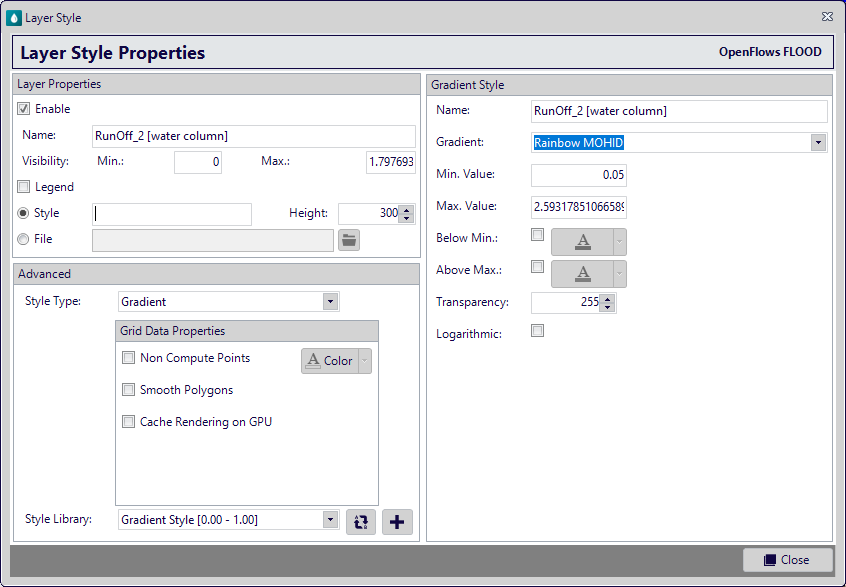
Figure 8 – Layer Style properties menu – configuring min. value to 0.05
If you use 0 or very small minimum values, since we are now simulating rain-on-grid, it’s difficult to interpret the results, because almost all grid cells will have at least a small amount of water in the surface.
As final result, in the time instant 2010-1-1 12:00, you should obtain something similar to this map:
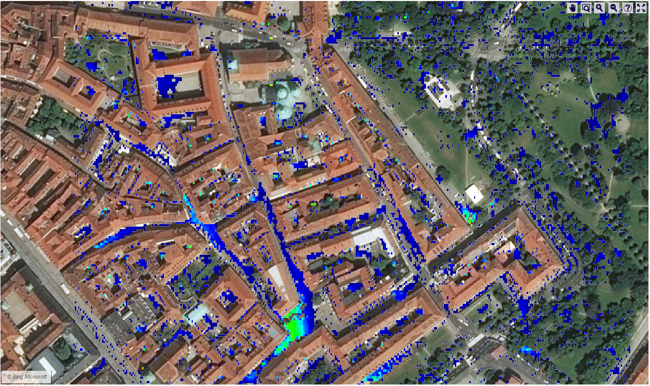
Figure 9 – Mapped output on water column for instant 2010-01-01 12:00 (simulation with direct rainfall)