| Product(s): |
WaterSight |
| Version(s): |
10.00. |
| Area: |
Documentation |
Overview
Investigate past, real-time and expected future performance for each asset using an embedded hydraulic model that is continuously updated with boundary conditions from sensors. The user is no longer limited by the number and location of sensors, being able to readily monitor several parameters at every point in the system.
One of the advantages of WaterSight is that it can automatically and continuously feed the hydraulic model boundary conditions with real time measurements from sensors (such as real time measured tank levels, real time measured pump status, real time measured PRV settings, etc) and also with real demand patterns, turning the traditional static hydraulic model into a much more accurate real time hydraulic model of the water system. In WaterSight the model will run automatically at a given frequency defined by the user, with a user defined hindcast and forecast period. For more information about feeding the hydraulic model with boundary condition from sensors, take a look at this article - Feeding the hydraulic model with real time measurements from sensors.
Prior to uploading a hydraulic model, review the tips and requirements described in WaterSight - Numerical Models article.
Layers
Use the layers option located on the top of the map to enable or disable additional geospatial information as well as the 3D context.
Any GIS information that is uploaded in WaterSight (through shapefile upload in the GIS administration page) will be here displayed.
Background: Allows to user to select the Background map to be displayed; Aerial, Hybrid, Street, None
Enabling 3D context: The 3D context includes the 3D terrain, the 3D building outlines. Both 3D terrain and 3D building outlines capabilities are automatically available for the region of interest. Building outline options only becomes available after you enabled the 3D terrain. To activate the 3D view, please use the shift + scroll button the mouse or use the rotate button located on the top right side to rotate the view  . More information here.
Model Element Visibility
The user can control the elements that are shown on the map, such as:
- Pipes - enable or disable pipes elements on the map view and which variables to see (diameter, flow, headloss, headloss gradient, velocity). Default is on.
- Junctions - enable or disable nodes elements on the map view, which variables to see (elevation, demand, hydraulic grade line, pressure). Default is on.
- Tanks - enable or disable tanks elements on the map view. Default is on.
- Reservoirs - enable or disable reservoirs elements on the map view. Default is on.
- Pumps - enable or disable pumps elements on the map view. Default is on.
- Control Valves - enable or disable PRV and FCV elements on the map view, and which status to see. Default is on.
- Isolation Valves - enable or disable isolation valves (TVC, GPV and Isolation valves elements) on the map view, and which status to see. Default is off.
- Customers - enable or disable customers elements on the map view. Default is off.
- Laterals - enable or disable laterals elements on the map view. Default is off.
- Flow Animation - allows the user to easily understand flow direction, through particles simulation.
Model Symbology
- Preset Map Configurations - controls the all model symbology and display:
- Default - Pipes Flow and Junctions Pressure are selected. Styles configurations can be configured by the user in the Administration, under Numerical Models.
- Low Pressures - Only Junctions with low pressures are displayed in the map. Styles configurations can be configured by the user in the Administration, under Numerical Models.
- High Pressure - Only Junctions with high pressures are displayed in the map. Styles configurations can be configured by the user in the Administration, under Numerical Models.
- Transmission Main - Only Pipes flow is displayed. Styles configurations can be configured by the user in the Administration, under Numerical Models.
- SCADA Elements - All sensors are displayed in the map
- Custom - Different model views can be configured and become easily accessible to operators. The user can select which variable to see for pipes and junctions. Styles configurations can be configured by the user in the Administration, under Numerical Models. More information here.
- Elements Outline - if enabled, all network elements are outlined in the map by a white contour line
- Pipes - allows the user to select which styles configuration to see in the map. Several styles configuration are automatically available by default such as: diameter, headloss gradient, flow, velocity, age and concentration. The user can change the defaults or add more. Styles configurations can be configured by the user in the Administration, under Numerical Models.
- Junctions - allows the user to select which styles configuration to see in the map. Several styles configuration are automatically available by default such as: age, concentration, elevation, HGL, pressure, Low pressure. The user can change the defaults or add more. Styles configurations can be configured by the user in the Administration, under Numerical Models.
- Control Valves - choose the control valves to display on the map: all, active, inactive or closed.
Map View
Map
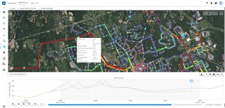
The default map view is an integrated view of the system, where hydraulic model elements are displayed together with the network sensors. When the model is first opened, it displays pipes colored by flow and nodes by pressure while the background is aerial view. The results correspond to the model run based on the most recent boundary conditions (e.g. pump status, tank levels) that have been imported from the SCADA system.
WaterSight can analyze both hydraulics and water quality parameters, such as age and concentration (for example chorine or any other constituent or contaminant). For both simulations (hydraulics and water quality) the conditions need to be first set up in WaterGEMS. For more information please take a look here, at the WaterGEMS Model Setup section.
The user can zoom in or zoom out using the scroll button of the mouse or using the "zoom" button located on the top right corner. It is also possible to navigate to any part of the network by moving the mouse while clicking at the same time in the scroll button (or by clicking in the "pan view" button located on the top right corner). Other options include the zoom extents view ("Fit view") and the button to select any element on the map in order to see the respective properties and results.
Direct measurements from SCADA or other telemetry systems can be used to set the initial conditions for the model run (initial conditions will be always imposed to the instant corresponding to the start of the simulation). More information here. Besides this, SCADA data can also be used to calculate each zone pattern, that can also be used to automatically adjust or calibrate the model demands, in case the Demand Adjustment option is enabled.
In the bottom of the page there is a time slide range bar that allows the user to navigate in the time history. Map results are updated accordingly whenever the user moves the time slide range bar backwards and forward in time. The "Map" marker on the graph allows the user to easily identify the time step that is being analyzed. The "Now" marker on the graph represents the local current time of the machine where WaterSight is running, and should match the current time at the water utility.

Model Element Graph
When clicking in any element on the map a table with the main properties and results of the selected element will pop up, together with a graph below.
Model element
For any hydraulic element selected (any pipe, node, pump, tank, reservoir, PRV or TCV) the graph view will display (at blue) the historical results, real time results and forecasts for the variables available, based on the hydraulic model calculations. The historical and forecast period duration is defined at the administration level, in the Numerical Models configuration page. The hydraulic model (WaterGEMS model) can be uploaded in the administration tab (Numerical Models configuration page) and will automatically run at a given (user defined) frequency.
Using the measurement dropdown located on the top left of the graph allows to change the measurement that is displayed in the graph for the specific selected element.
Model element associated with sensor
The model elements that also have real sensor measurements associated are represented in the map with a wi-fi symbol. When clicking in one of these elements, two lines will be displayed in the graph: black line corresponding to the sensor measurement and the blue line corresponding to the model result. Directly comparing these two lines at some points of interest allow the user to understand how calibrated and accurate the model can be.
Using the measurement dropdown located on the top left of the graph allows to change the measurement that is displayed in the graph for the specific selected element.
Checking model accuracy - checking boundary conditions
The user can easily check model accuracy by directly comparing how modelled data differs from the measured data.
Click in the hydraulic model element that has associated a sensor (represented by a wi-fi symbol) and analyse the graph. When selecting the model element, please also make sure that the graph is related to the modelled parameter for which sensor measurements also exist (in the dropdown with the available parameters, select those that have a wi-fy symbol) - see figure below.
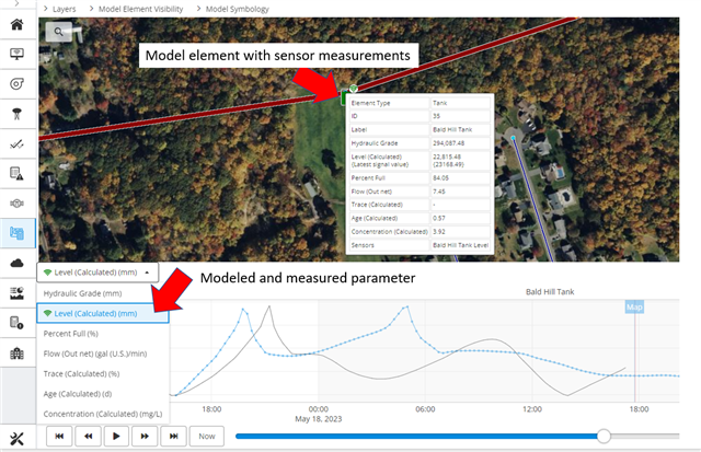
The black line corresponds to the sensor value while the blue line corresponds to the calculated result from the model. If both lines are near each other, a good fit between modelled and measured data was achieved for that location. Otherwise, further investigation and additional model calibration may be required.
Another important note: if the black and the blue line match the exact same value for the initial time step of the model run (when the blue line starts), then it means that sensor data is being used to set the initial conditions for the model run. In case there is a gap between the value for the initial timestep of the model run and the sensor data, then the sensor data is not being used to actively set the initial conditions of the model.
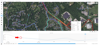
Figure 3. Sensors data being successfully used as initial conditions for the model run.
The sensors measurements that can be used to override the initial conditions of the hydraulic elements are the following:
- Tanks: level or hydraulic grade
- FCV: flow setting
- PRV, PSV, PBV: pressure or hydraulic grade
- Pumps: relative speed or pump status
More information how to setup, here.
See also
Hydraulic model setup
Imposing Initial Conditions from SCADA to the Model
Automatic Demand Adjustment
Automatic Hydraulic Grade Adjustment
OpenFlows WaterSight TechNotes and FAQ's
