Questions about this article, topic, or product? Click here.

WaterSight - Numerical Models

Product(s):	WaterSight
Version(s):	10.00.
Area:	Documentation

Note: It is highly recommended to turn off and delete track changes in the WaterGEMS model prior to upload in WaterSight (more information below) and also to upload a zip extension file (with just the sqlite extension) for performance reasons.

Overview

This administration page is used to upload the hydraulic model and set the options for the automated real time simulation.

Sensors measurements can be used as boundary conditions for the hydraulic model runs, contributing to increase the confidence in the model calculated results (such as tank levels, PRV settings, pump status and relative speed, etc). Besides this, zone patterns and hydraulic grade line patterns for tanks and reservoirs can also be used as boundary conditions for the model runs, but in this case they are not applied only for initial conditions, but rather to the all simulation period. More information can be found here.

The uploaded WaterGEMS model will automatically run in WaterSight, at a given frequency defined by the user and also considering the hindcast and forecast period defined (more detail below). If the WaterGEMS model contains more than one scenario, only the active scenario will be considered in WaterSight.

General Tips

In order to successfully run the hydraulic model in WaterSight, the user should first check if the EPS model is successfully running in WaterGEMS. In case there are errors, the user should first correct them using WaterGEMS. To take full advantage of WaterSight capabilities, the user should check if the WaterGEMS hydraulic model is updated with all relevant network elements (all linear and vertical assets). Some tips below:

customer meter elements are updated and, ideally, the billing ID field in the model matches the ID provided in the Customer Meter and Billing configuration files (customers will be used in the Pipe Break, Fire Event and Pump Shutdown workflow),
all isolation valves are updated (will be used in the Pipe Break workflow). The user can use TCV, GPV or isolation valves types in WaterGEMS to represent the operating valves in WaterSight;
all SCADA elements are created and mapped to the respective model elements (this is important to assure that model boundary conditions are being fed by real sensors measurements. Both name of the SCADA signals and units need to match those defined in WaterSight. More information here),
when using the automatic demand adjustment option of WaterSight (see below for more information) it is required that the zones name in the WaterGEMS hydraulic model are associated to the nodes and match the names given to the zones in WaterSight.
the tank definition in the model must match the SCADA type. If the SCADA signal is Level, the tank "Operating range type" should be defined by Level. If HGL, then tank Operating range type" should be defined by Elevation.
for performance reasons, please make sure that you delete all track changes from the WaterGEMS model. To delete track changes go to the review tab in WaterGEMS >> select Bulk Archive >> delete records (see image below). After that, please make sure to compact database, by acceding to File >> Database utilities >> Compact Database. At the end, make sure to save the file. This workflow can significantly reduce the size of the SQLite file in case the utility is using the track change functionality quite often.


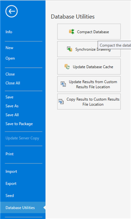Delete track changes in the WaterGEMS model	Compact database in the WaterGEMS model

WaterSight can also display water quality results such as age and constituent analysis. In case of a constituent analysis the user needs to define the constituent properties and the concentration at the sources in the WaterGEMS model. More information about the workflow to set up age and constituent analysis in WaterGEMS, take a look here. For more detailed information about defining constituent properties in WaterGEMS, take a look at this article. Please note that to see water quality results in WaterSight the calculation type in WaterGEMS needs to be set to "Age, Constituent & Trace" as mentioned below. Also make sure to define a trace node in WaterGEMS (like for example a tank or Reservoir) otherwise the model will not run.
Only one hydraulic model file is supported by digital twin, however in case the water utility has several model files of distinguish areas and pretends to upload into one single digital twin, it is possible to aggregate those into one single model file by using the Import submodels functionality of WaterGEMS. To do that open one of the WaterGEMS file, go to File >> Import >> Submodels and add the second SQlite file. Please note that in case there are errors while importing the submodel, most likely that both submodels have duplicated element labels. In that case make sure to rename pipes labels and/or junctions labels and/or other element labels. This can be quickly achieved using the relabel function available from the flex tables (when clicking with the right button of the mouse over the Label column header). Also make sure that, prior to merge the models, that in both models the demand alternative has the exactly same name, so that both can be considered. More information here.

Two submodels uploaded into WaterSight

WaterGEMS Model Setup

Required Settings

If the WaterGEMS model contains more than one scenario, only the active scenario will be considered in WaterSight. Be sure the appropriate scenario is set as active and save the file prior to uploading.
Update the calculation within WaterGEMS. Go to Home >> Options and procede with the following additional configurations:
- Calculation Type: SCADAConnect Simulator
- SCADA Calculation type: "Hydraulics only", if only running hydraulics; "Age, Constituent & Trace" if running both hydraulics and water quality analysis
- Simulation mode: needs to be set to Historical

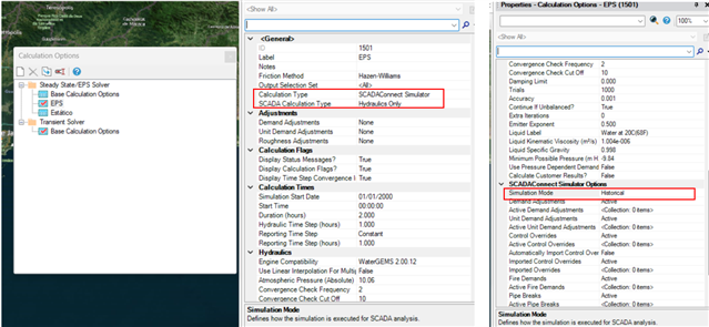
Figure 1 - Updating calculation options in the WaterGEMS prior uploading into WaterSight.

Once done, make sure that the model successfully computes in WaterGEMS with no errors. If there are errors the user will need to fix those before uploading the model in WaterSight.

Recommended Settings - Set initial conditions for the model runs based on real measurements from sensors

SCADA or other telemetry data can be used to set the initial conditions for the model run when they are correctly configured in the uploaded WaterGEMS model. More information here.

WaterSight Hydraulic Model Fields

Click in the "Add" button (+) located on top to add a new hydraulic model.

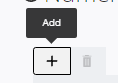
Tips: Only one hydraulic model file is supported by digital twin however it is possible to aggregate several model files into one using the import submodel feature available in WaterGEMS. More information above, under General tips. To upload a new model file, it is strongly suggested to upload a ZIP extension (just including the sqlite extension) and to turn off and delete track changes

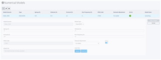
Once clicking "Add", the following fields become available:

Model Domain

Internal model ID generated by the system once the model is uploaded.

Model Type

Model input format. For now it is only possible to upload WaterGEMS models.

Spinup (h)

Time period at the start of a model run where the results are considered unstable and are not displayed. This is particularly important for model runs where initial inertia is important. For water supply models spinup this can be relevant when simulating water quality. In most cases this value can be set to 0, as consecutive model runs use previous results to update initial settings.

Hindcast (h)

The Hindcast is a time period of time leading up to the current time where past model calculated results can be compared with historical sensor values. A hindcast period of 12-24 hours is useful for calibrating and validating a near-realtime hydraulic model, as well as in giving context to current and forecast conditions. If the model is configured with Control Overrides from SCADA sensors, a hindcast period can have accurate behavior of pump and valve setpoints even if logical controls have not been fully defined in the model.

Forecast (h)

The time period into the future, starting from the current time, for which model results will be calculated. Note that the forecast period cannot take advantage of SCADA Control Overrides, so controls must be defined in the model which appropriately mimic both automated setpoints and typical manual adjustments to pump and valve operations. When first developing a near-realtime hydraulic model, it is often best to focus first on calibrating an accurate hindcast, and then refine controls to improve the forecast.

Results of each model run are automatically saved in the Previous Simulations page.

Run Frequency (h)

Define the automatic run frequency of the model. For example if 1 hour is defined, this means that the model will automatically run every hour.

EPSG code

EPSG (European Petroleum Survey Group) code of the WaterGEMS model. This is required in order to have the model displayed in the correct position in the map. In most cases, the EPSG code or a description of the coordinate system can be found by examining the layer properties in any GIS software. Note that each layer may have different coordinate systems if the utility has not standardized to a single system. EPSG codes can be found by searching https://spatialreference.org/.

In case there is an error during the model upload process or in case the model is based on an ESRI code (instead of EPSG code), the user has the possibility to define the WKT (well-known-text) for that specific EPSG / ESRI code that is not supported. For more information click here.

After defining a EPSG code, to change it again the user will need to reupload again a hydraulic model.

Demand Adjustment

Select the demand adjustment options that will be automatically applied by WaterSight:

No Update:

This means that WaterSight will use the same exact demand values defined in the WaterGEMS uploaded model, including all base demands and unit demands, demand multipliers (patterns) and other demand adjustments defined by the user.

Update Demand & Patterns (Global):

WaterSight will automatically compute a global pattern for the entire system, and will automatically apply this global pattern to all nodes of the network. The total demand for each node is obtained by adding up all base demands and unit demands (unit demands multiplied by number of units) defined in the WaterGEMS model and then by multiplying this final node demand by the global pattern automatically computed by WaterSight.

The global system pattern is automatically calculated by the software and takes into consideration the following:

The global system zone flow corresponds to the sum of all inflows, subtracted by all outflows, and by taking into account also the storage variation inside the system;
Last month of historical zone flow data is used to calculate a pattern for the global system zone (dimensional values);
Global pattern, including a one week forecast, is calculated using a machine learning algorithm, together with advanced data analytics methods. Bad data, including outliers and spikes are removed from the analysis and a different pattern for week days and weekends is computed;
Global pattern with dimensional values is transformed into a global multiplier (or dimensionless pattern) and applied to each node of the model;

To assure that a global pattern is calculated, all inflows, outflows and storage sensors for the system total zone must be defined (information configured in the Zones configuration page) and transmitting data into WaterSight (make sure sensors are defined in the Sensors configuration and that the On-Premise tool (OFOSC) is working).

The global system dimensionless pattern (global demand multiplier) covers all simulation window period defined by the user in the Numerical model settings (hindcast + forecast). The global dimensionless pattern also differentiates between weekday, Saturday and Sunday. For example if the simulation window covers a Friday and a Saturday, the global demand multiplier for Friday and Saturday will be quite different.

Another important aspect to mention is that the global pattern is continuously and automatically being updated in real time (whenever new data arrives into WaterSight) using always last month of historical data. This means that the global pattern for today is slightly different than the global pattern of the previous day and will be slightly different from tomorrow global pattern.

Update Demand & Patterns (Zone-by-Zone)

WaterSight will automatically compute a pattern for each zone (according to each zone defined in the Zones configuration page), and will automatically apply each zone pattern to the nodes belonging to the respective zone. For this to happen it is necessary that the zones name in the WaterGEMS hydraulic model (and associated to the nodes) match the names given to the zones in WaterSight (zone names are configured in WaterSight by changing the zones information contained in the shapefile that is uploaded in the GIS configuration page). For the model nodes with no zones assigned or with zones different that those defined in WaterSight, patterns and demand adjustments will be ignored (only base demand and units demands will be taken into account).

The total demand for each node is automatically obtained by adding up all base demands and unit demands (unit demands multiplied by number of units) defined in the WaterGEMS model and then by multiplying this node final demand by the respective zone pattern.

The zone pattern is automatically calculated by the software following the same methodology used for global system pattern explained above:

Each zone flow corresponds to the sum of all inflows, subtracted by all outflows, and by taking into account also the storage variation inside the zone;
Last month of historical zone flow data is used to calculate a pattern for each zone (dimensional values);
Each zone pattern, including one week forecast, is calculated using a machine learning algorithm, together with advanced data analytics methods. Bad data, including outliers and spikes are removed from the analysis and a different pattern for week days and weekends is computed;
Each zone pattern with dimensional values is transformed into a zone multiplier (or dimensionless pattern) and applied to all the nodes that belong to the respective zone;

The zone dimensionless pattern (zone demand multiplier) covers all simulation window period defined by the user in the Numerical model settings (hindcast + forecast). The zone dimensionless pattern also differentiates between weekday, Saturday and Sunday. For example if the simulation window covers a Friday and a Saturday, the zone demand multiplier for Friday and Saturday will be quite different.

Another important aspect to mention is that zones pattern are continuously and automatically being updated in real time (whenever new data arrives into WaterSight) using always last month of historical data. This means that the zone pattern for today is slightly different than the zone pattern of the previous day and will be slightly different from tomorrow pattern.

To assure that a zone pattern is calculated, all inflows, outflows and storage sensors must be defined (information configured in the Zones configuration page) and transmitting data into WaterSight (make sure sensors are defined in the Sensors configuration and that the On-Premise Data Pusher tool is correctly working). Besides this, to assure that a reliable pattern is computed, all zone boundary valves should be closed and zones should be as stable as possible throughout the year (frequent change of zones boundaries affect pattern reliability).

The user can analyze each zone dimensional pattern automatically calculated by WaterSight by acceding to the Zone details graph (under Network Monitoring page). Once in the zone detail graph, the user should change the interval to "15 min" and the pattern dropdown option to "Last month" and enable the legend by clicking on the existent button on the top right of the graph.

Then disable on the graph all pattern confidence bands (5/95 band and 20/80 band) and the real time series, and keep only the median series (P50 Average). This is the dimensional pattern that will be automatically transformed into a dimensionless pattern (zone demand multiplier) used to multiply all existent node demands of the hydraulic model, in case this option is enabled in the Numerical Model settings. The user also has the option to export the zone dimensional patterns to CSV by clicking in the Download button located on the top right of the graph

In case the user defined patterns in the original WaterGEMS uploaded model are not very accurate (for example the patterns are not updated or were developed based on reference values, etc) or if no patterns at all were defined in the original WaterGEMS uploaded model, then the automatic adjustment options available in WaterSight can significantly improve the accuracy of the model.

In the example below, tank level results (modeled VS SCADA) are compared using the two different demand adjustment options available: Global Demand Adjustment and Zone Demand Adjustment.

Global Demand Adjustment

Zone Demand Adjustment

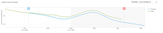Figure 2. An example where tank level results (modeled vs SCADA) were compared using different automatic demand adjustment options available in WaterSight.

Some additional information can also be found here.

HGL Adjustment

Enable or disable Hydraulic Grade adjustment for each reservoir model element. This feature is particularly useful when using hydraulic models of distribution systems that do not cover the transmission line.

Hydraulic models of distribution systems commonly have reservoirs elements representing DMA's inflow node (such as storage tanks). In that case, model's scope doesn´t cover the transmission line of the network that feeds the DMA, and usually a virtual reservoir is placed as starting point.

Whenever this happens, and instead of assuming a fixed hydraulic grade for the reservoir for the all period of the simulation run (corresponding for example to simulate the tank always full or always with an average level), WaterSight can forecast the real level of the tank and based on that calculate a pattern that can be applied to any reservoir model element in order to simulate the correct pressure levels at the boundary condition, for the all period of the run (and not only as initial conditions).

In order to be able to enable or disable HGL adjustment for each reservoir, it is required that the hydraulic model contains at least one reservoir as model element with an associated hydraulic grade signal. The hydraulic grade signal needs to be created/added both on the WaterGEMS file and also uploaded in WaterSight, through sensor administration. For more detailed information on the specific steps to set up this, please take a look at this article - Automatic Hydraulic Grade Adjustment.

Please note that the real-world upstream element may not be a tank, it may just be a pipe that connects a complicated upstream network that is not part of the model. So the real-world sensor might be a level, or it might be a pressure, or it might even already be an HGL. For all those cases, this feature can be applied, following the steps mentioned here - Automatic Hydraulic Grade Adjustment.

Active

Turn the model active or inactive. If inactive, the hydraulic model will not appear in WaterSight and the Modeling section will not be available.

Valve Display

Display GPV as

In case user uses GPV valves in the WaterGEMS model file, those can be considered in WaterSight as Isolation Valve (default) or as Control Valve. In case they are considered as Isolation Valve, they will appear in the Current Simulation page under the Isolation valve group dropdown. In case they are considered as Control Valve, they will appear under the Control Valve group dropdown.

Display TCV as

In case user uses TCV valves in the WaterGEMS model file, those can be considered in WaterSight as Isolation Valve (default) or as Control Valve. In case they are considered as Isolation Valve, they will appear in the Current Simulation page under the Isolation valve group dropdown. In case they are considered as Control Valve, they will appear under the Control Valve group dropdown.

Allow valve status update through API

Making sure that valve status in WaterSight are updated is very important to achieve good confidence on the model results. With WaterSight it is possible to directly and automatically update valve status for example based on the latest GIS information, through an API. For more information, please contact your Bentley technical support person.

Upload

Click here to directly upload a WaterGEMS model - can be sqlite file or ZIP file extension. To assure a fastest upload, it is strongly suggested to use the ZIP extension (just including the sqlite extension) and to turn off and delete track changes in the WaterGEMS model. The upload Model button should also be used for further reuploads of the hydraulic model.

Styles

Manage the color coding configuration for the model. More information here.