Questions about this article, topic, or product? Click here.

Using Darwin Calibrator

Product(s):	WaterGEMS
Version(s):	CONNECT Edition, V8i
Area:	Modeling

Overview

The purpose of this technote is to explain how to calibrate a model using Darwin Calibrator in Bentley WaterGEMS. Additional information can be found in the WaterGEMS Help menu.

A video demonstration can also be found on the Bentley Hydraulics and Hydrology Modeling YouTube Channel: Automated Calibration with Darwin Calibrator in WaterGEMS

NOTE: before attempting to use Darwin Calibrator, it is strongly recommended that you review Water Model Calibration Tips

Background
Setting up a Calibration Study
Manual Calibration Run
Optimized Calibration Run
Updating the Model
Tips
Importing Field Data from SCADA
Troubleshooting
- Matching model results with Calibrator
- Calibrator User Interface Sluggish

Background

Darwin Calibrator

In order to accurately model a water system, the user will often need to calibrate the model. Darwin Calibrator allows the user to calibrate a model either manually or, with efficient genetic algorithms, in a more automated fashion. It allows for multiple calibration candidates to be presented so the best possible solution to a given system can be found. Solutions can also be exported into a new scenario for use in an existing water system.

Licensing

Darwin Calibrator is included with a license for Bentley WaterGEMS. Older licenses for WaterCAD allowed for the purchase of Darwin Calibrator as a separate add-on. This is no longer available but has been grandfathered in for these licenses. As of version 10.03.02.75, Darwin Calibrator is still available in the menu inside WaterCAD so that those who had purchased Calibrator separately in the past (and those who have Calibrator as part of also having WaterGEMS) are able to use it. If you only have a license for WaterCAD and had not purchased a separate Calibrator license in the past, you will only be able to perform Manual runs inside Calibrator (not optimized runs). You would need to upgrade to WaterGEMS (which can open WaterCAD models) to use optimized runs in Calibrator.

Note: for versions that use SELECTserver licensing (below version 10.02.XX.XX) Non-SELECT users will need to check out both WaterGEMS and Darwin Calibrator in order to use this tool. You can check out the license from the License management tool.

Calibration

Before using Darwin Calibrator, it is important to keep in mind that there are two main steps to model calibration when the original model does not agree exactly with the field data:

Determine WHY there is a discrepancy.
Make the necessary adjustment

Darwin calibrator can work very well for #2, but the vast majority of the work is in #1. Before using Darwin Calibrator, it is best to make several model runs trying to get your best answer and understand the sensitivity of the model to parameter changes. There are a number of papers and scholarly articles about model calibration, available online and in popular water resources journals.

Setting Up a Calibration Study

In order to calibrate a model, Darwin Calibrator makes adjustments to the pipe roughness, demand, and/or element status. For this reason, the first step for any calibration study is to have a completed model with all demand and roughness data entered.

With a completed model ready, you are set to start using Darwin Calibrator. You can open Calibrator by going to Analysis > Darwin > Darwin Calibrator, for Connect Edition versions. In the V8i releases of WateGEMS, you would go to Analysis > Darwin Calibrator.

The Darwin Calibrator window will then open.

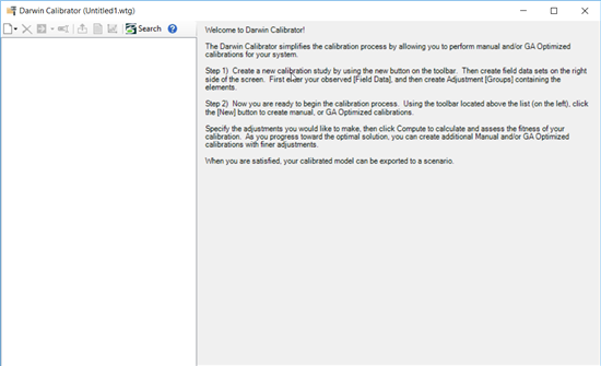
To start a new calibrator study, select the New icon in the upper left and select New Calibrator Study. You will then see tabs and available features appear on the right part of the window.

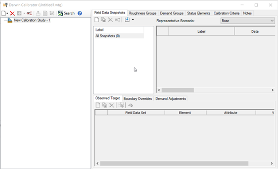
The next step is to create your adjustment groups. Adjustment groups are groups of elements whose attributes can be adjusted together during the calibration process. (all elements in the group are adjusted by the same amount). So, they would typically be things where there is a degree of uncertainty and you would like Calibrator to be able to adjust the value in order to try to get the model results to match the field measurements. You must be careful to group similar elements and not dissimilar ones. It is recommended to group elements together who have similar properties. You can adjust the properties for a group as a whole but not for individual members of the group. While you can also set up the field data snapshots, it is recommended that the adjustment groups are created first, rather than let available data determine how many adjustment groups to have. For clarity, the focus will be on creating roughness groups, though the general steps will be the same for demand groups and status groups.

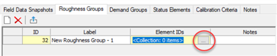
Go to the Roughness Groups tab. Click the New icon to create a new item. It is up to the engineer how many groups to create. The recommended workflow is to group elements that have similar characteristics such as age or material, since it can be assumed that two pipes of the same age or material will see similar changes to the actual roughness (as again, all elements within the groups are adjusted together, not individually). To add elements to the roughness group, click the cell in the Element IDs column and select the ellipsis button.

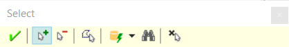
A new window will open. Choose the “Select from Drawing” icon.

The Select toolbar will appear, allowing the modeler to choose elements from the drawing using a few different ways, including manual selection and query, among others. Once you have the elements selected, click the green check mark to complete the selection.

You will now see the elements in the table. Click Okay to return to Darwin Calibrator.

The selection of Demand and Status groups follow similar steps. Click the in the Demand Group or Status Element tab to select the elements same as explained above.

Note: Status Elements are used when you have a degree of uncertainty of the status of the element, such as a valve that may or may not be stuck. It is recommended that Status groups contain one or very few pipes.

With the adjustment groups selected, now it is time to enter the field data snapshots. Return to the Field Data Snapshots tab. Make sure the representative scenario is set to the one to be used in the calibration study. Darwin Calibrator will pull results from a given scenario to compare to the adjusted values from the calibration study.

Next, select the New icon below the Field Data Snapshot tab. You will see a new field data snapshot appear.

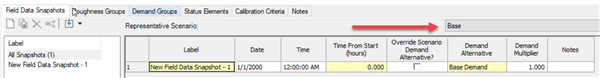
For the "Date" and "Time" field, enter the respective date and time when the measurement(s) were taken. Be sure that your scenario's calculation options are also set to the right date and time as well - this way it will use the correct demand pattern multipliers and indicate the correct "time from start" (which shows the difference between the scenario's start date/time and the field data snapshot's date/time).

Also, identify a demand multiplier, if necessary. For example, if you have knowledge that your demand is higher or lower by a specific percentage, you can set that value here. The default value is 1.

Next, the observed data for the field data snapshot will need to be entered. This is entered in the lower right of the window, below the Observed Data tab. With the field data snapshot highlighted, click the New button under the Observed Target tab. A new line will appear with the Element cell blank.

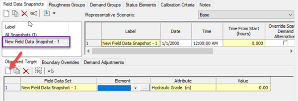
Click inside the cell, and then click the ellipsis button. Select the element that you have the data for from the drawing or use the Find option. Once you have selected the node, it will be available in the pulldown. With the node selected, the Attribute and Valve columns will be editable. Choose either Hydraulic Grade or Pressure for the attribute and then enter the appropriate value. Enter as many elements as you have field data for.

If you have a field data snapshot for another time during the model run, you can create a new one with a different time. You can then enter observed data for this time as well.

You can also import the field data using Modelbuilder or SCADA, if you have data for multiple elements at multiple times. Steps are importing field data are explained in the help documentation and in this article: Importing Darwin Calibrator Field Data using ModelBuilder

Next to the Observed Data tab is the Boundary Overrides tab. This is also important in a calibration study since it is possible that a tank level or pump/valve status is different from how it is depicted in the model. To get the most accurate results, applicable boundary overrides should be applied.

Click the Boundary Override tab and select the New icon below the tab. A new item will appear, you need to select the feild data snapshot for which you want to apply the boundary override. Select the element as before, keeping in mind that this should be a tank, valve, or pump. Depending on the element chosen, the Attribute field will offer different selections. For a tank, the Attribute can be either Hydraulic Grade or Tank Level. For pumps and valves, setting and status are the options. Again, enter the appropriate value for the attribute selected.

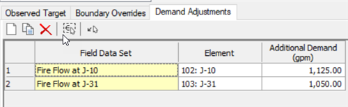
Demand Adjustments is the last tab. This is used to adjust demand for individual elements, such as flow from a hydrant or a junction that occurs only during the time that the field measurements were observed. Enter data here as necessary. Note that the "simulated flow" results at the end of the calibrator run do not list demand adjustments - you can assume that the demand adjustment values that you enter will always be applied during the timestep specified in the field data snapshot during calibration (assuming that you have chosen to use the snapshot in question in a Calibration run).

Manual Calibration Run

With the field data and boundary overrides entered, and the adjustments groups created, you are ready to run a calibration study. This section will discuss the manual calibration run. As before, the steps below will show a calibration study using roughness adjustment groups. Similar steps can be taken with demand groups.

The manual calibration study allows the user to enter multipliers or set values to change the existing roughness coefficient of pipes, demand, or status to a new value or to conduct the leakage detection study. After computing the study, you can compare the simulated results to the field data entered that given time.

To start a new manual run, click the New icon in the upper left and choose “New Manual Run”. A new item will appear below the calibration study label. On the right side of the window will be a series of tabs. In the roughness tab, you will see the roughness groups created earlier. To make a certain roughness group active, make sure the check box under “Is Active?” is checked. For the Operation column, choose either Multiply or Set, depending on which you wish to use. For Value, enter the appropriate value. Then click the Compute button.

Note: Multiple manual runs can be created so that a number of values can be entered for the roughness.

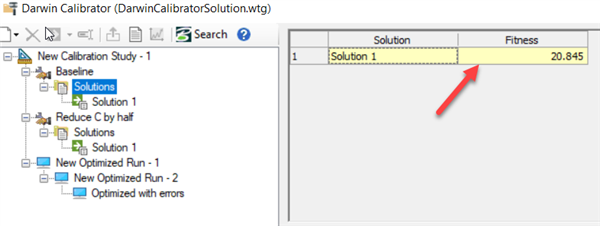
When completed a solution will appear that will include the results from the calibration study. Click “Solutions” directly under the manual run. This will display a fitness value for the solution or solutions. Fitness is a correlation between the observed data from the field data snapshot and the calculated value from the calibration study. The smaller the value, the better the fit.

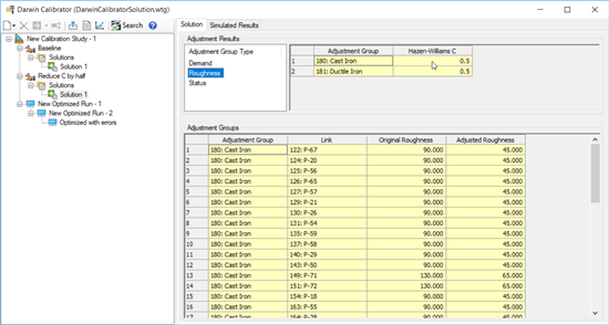
Returning to the left side of the window, click “Solution 1” to view the results. Under the Solution tab will be the adjusted roughness values for the pipes included in the calibration study. Under the Simulated Results tab will be the elements included in the field data snapshots. (the observed pressure/flow, not the status or demand adjustments) Columns for the observed data and the simulated data with the new roughness coefficients are presented, along with a column showing the difference between the observed and calculated values.

Optimized Calibration Run

The optimized calibration study uses a genetic algorithm to find the best possible solution available within certain parameters. The optimized calibration study has no true optimality and only knows the best solution relative to other solution already found during computation. However, the optimized calibration study runs through a large number of possible solutions and can often find a very good solution to fit the model.

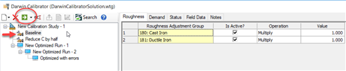
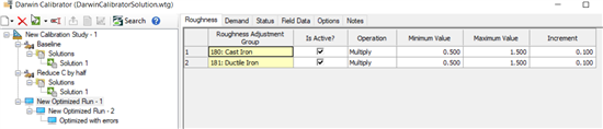
The process is similar to the manual run. Click the New icon in the upper left and choose New Optimized Run. Under the Roughness tab, you will see the roughness groups created earlier. To make a certain roughness group active, make sure the check box under “Is Active?” is checked. For the Operation column, choose either Multiply or Set, depending on which you wish to use. Instead of entering a new value manually for the roughness, you will enter minimum and maximum values, as well as an increment. Then click the Compute button.

Darwin Calibrator will then try different values for roughness that fall within the values entered in the Roughness tab and compare the resulting values to the observed data from the field data snapshots. Darwin Calibrator will continue this until it finds the best solution available. The results are viewed just as the manual run, however there is an option to view as many as ten solutions. See the Tips section below for more information about this.

Updating the Model

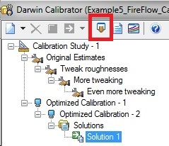
If you are satisfied with the results, you can export the new roughness coefficients, demands, or status to a new physical alternative. To do this, highlight the solution you wish to export. The “Export to Scenario” icon will become active.

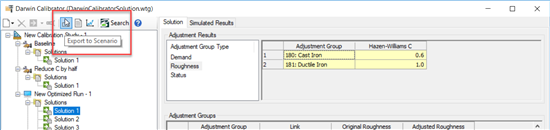
Choose this icon and a new window will appear.

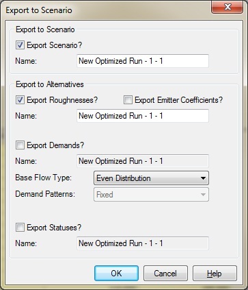
To export to a new scenario, check the “Export to Scenario?” box. Do the same for the alternatives. With the check boxes selected the new results will be exported to new physical or demand alternatives (depending on the type of calibration study done). If you export to a scenario and do not export to an alternative (by unchecking the associated box or boxes), the data for that alternative type will be exported to the Base alternative.

Note: The data in your original model will not change unless you use this export feature.

Tips

For performance-improving tips, see: Darwin Calibrator Performance Improvement Tips for Large Models
For general tips, read the Help topics "GA-Optimized Calibration Tips" and "Darwin Calibrator Troubleshooting Tips".
After computing a calibration study, you will sometimes see results that do not have a good fitness or do not make sense. Below are a few general tips to look at. More information on Darwin Calibrator can be found in the WaterGEMS Help documentation.
- Try running a manual calibration study with no adjustments to the roughness or demand. In other words, keep the multipliers for the adjustments groups at 1. Then look at the fitness. If you have a very high fitness number, this is an indication that something is wrong with the model setup. Review your model and make sure the results look reasonable and that no unusual user notifications are generated.
- Verify that the boundary overrides and demand adjustments are properly entered. This is very important since otherwise Darwin Calibrator will use values in the model at the times of the field data snapshots instead. Since the results in the model results might not be the same as what is actually occurring in the field, it is important to make these changes. Accurate data model-wide is important as well. Good, accurate data will mean the calibration study will work optimally.
Using field data that includes a higher flow tends to allow you to find better results for the roughness coefficients. With higher flows, you have higher velocity results. Because of the structure of the Hazen-Williams equation, this will allow you to have a larger spread in C values for a difference in pressure.
If you are computing an optimized run, you can change some of settings in the Options tab. Highlight the optimized run on the left side of the window, then choose the Options tab on the right. Detailed information for the options can be found in WaterGEMS Help. Changing the Maximum Trials and the Non-Improvement Generations items to higher values will allow Darwin Calibrator to try more adjustments and possibly find better solutions. You can also change the Fitness Tolerance and the Solutions to Keep. It is recommended that the Advanced Options remain set to the default values.
Since Darwin Calibrator’s genetic algorithms can only compare a result to results that came before, making changes to the options can create new sets of solutions. It is recommended that you run several optimized runs even if the initial calibration study is good. A better solution might be generated after changing the parameters.
WaterGEMS and WaterCAD also come with several sample models that have completed manual and/or optimized calibration studies. These are a good resources to see the general setup of a calibration study, and can allow you to calculated models and see how the results differ not only with between manual and optimized runs, but also in changing the options. The sample files can be found at the following file path. C:\Program Files (x86)\Bentley\WaterGEMS\Samples
Example5.wtg is an example of calibration based on three hydrant flow tests done at different times of the day. The hydrant flow, pressure, and corresponding pump and tank status are shown in the Demand Adjustments, Observed Target, and Boundary Overrides tabs within the calibration study, respectively.
Example4.wtg shows a system separated into DMAs, demonstrating the use of the Pump Station element. A Darwin Calibrator study is included, giving examples of calibration based on both static and residual hydrant flow tests. Optimized runs where both demand and roughness can be adjusted are included, along with examples of Manual runs where roughness and/or demands are adjusted manually.
Example8.wtg is an example of a leakage detection study using Darwin Calibrator. Observed hydraulic grades at several different locations in the system have been entered, for several different times of the day. The "Detect leakage node" option is used in each of the optimized runs, to detect leakage node candidates by using emitters.

Importing Field Data from SCADA

A new option in WaterGEMS V8i SELECTseries 5 and later allows the user to import field data directly from your SCADA data right in Darwin Calibrator. You click the "Import Field Data from SCADA" button to do this.

You can then select data to import into Darwin Calibrator. Note that there is no bulk import tool, but you can easily import representative data to use in model calibration.

How do I match the results I am getting from Darwin Calibrator in my model?

In order to match the results that you are getting from Simulated Results tab in Calibrator (see image below) you will need to do the following:

1. Make sure the scenario you are look at in your model is the representative scenario listed in the Field Data Snapshots tab
2. Make sure the calculation options (Analysis > Calculation Options) for your scenario are set to represent the field data snapshot you are looking at results for.

Calibrator only calculates results for a steady state scenario at a particular time period that you specify in your field data snapshot so it only makes sense to set your model up to reflect this. In this example we are looking at the field data snapshot labeled “Flow Test 1”

NOTE : If you want to run Darwin Calibrator for EPS analysis, then you would need to use a particular time-step from EPS, which will work as steady state calibration.

In your model you will need to set your calculation options as follows:

Simulation Start Date = The same date listed in the field data snapshot
Time Analysis Type = Steady State
Is EPS Snapshot? = True
Equivalent Hydraulic Time Step (hours) = 1.00
Start Time = The same time list in the field data snapshop

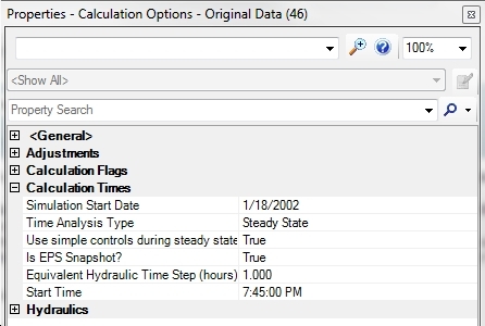
Setting the calculation option for “Is EPS Snapshot? = True ensures that your model is going to use the pattern multiplier that Calibrator used when doing its calculations.

3. Make sure ALL the boundary overrides, for the particular field data snapshot you are looking at, are reflected that way in your model. For example, if you have pump PMP-1 set to a status of ON in your boundary overrides tab make sure your model has this pump set to a status of ON too.

4. Make sure that if you have any demand adjustments set that you also add those into your model. Demand adjustments are in addition to current demands already in your model when you run Calibrator, they are not in lieu of them. For example, if you have a demand adjustment of 41.01 L/s on junction J-170 then you would need to make sure to add that to J-170’s demand collection in addition to what is already there for that junction when Calibrator was run.

5. After you run Calibrator and are happy with the solution make sure you export that solution. In order to achieve the same results in your scenario you will need the adjusted values that Calibrator arrived at for your roughness adjustment groups, demand adjustment groups, and status elements.

After you make all these changes to the scenario in your model just compute and look at the properties of the observed target in your model to make sure it matches the simulated results in Calibrator.

Navigating Calibrator is very slow / sluggish in some large models

When working with a large model, you may notice long delays in clicking between tabs or otherwise sluggish performance navigating the Calibrator user interface, especially when using "all snapshots".

This was a known issue in version 10.03.02.75 (reference # 572435), which has been resolved in a cumulative patch set. Please contact Technical Support for the patch, or upgrade to a newer version when available (as it will include the fix).