Questions about this article, topic, or product? Click here.

Running a Long Term Continuous Simulation

Applies To
Product(s):	CivilStorm, SewerGEMS
Version(s):	CONNECT Edition, V8i (SELECTseries 2) or later
Area:	Modeling
Original Author:	Scott Kampa, Bentley Technical Support Group

Overview

The purpose of this TechNote is to discuss the Long Term Continuous Simulation (LTCS) function available in CivilStorm V8i SELECTseries 2 and SewerGEMS V8i SELECTseries 2 and later.

Background

EPA SWMM has the capability of running long term continuous simulations, but previous builds of CivilStorm and SewerGEMS were mainly designed for computing event-based simulations. CivilStorm and SewerGEMSV8i now include the capability of running such a simulation. The CONNECT Edition releases and any release later than V8i SELECTseries 2 include this feature.

Long Term Continuous Simulation will use data such as rainfall, temperature, evaporation, infiltration, snow packs, as well as aquifer and groundwater data. While it is possible to compute with the Implicit engine, it is designed for use with the Explicit (SWMM) engine, which is better at handling the large amounts of data goes into such a simulation.

Furthermore, when using catchments and rain file data, the EPA-SWMM runoff method must be used.

This TechNote will review the data needed to complete the simulation and the steps to successfully run the model.

Rainfall Data

Where CivilStorm and SewerGEMS used storm data such as Time-Depth curves or IDF tables to define a storm event, a new item called “Rain File” is included for use of historical data used in LTCS. These files can come in a number of different allowable formats. For details on the supported formats, see: Entering Known Rainfall Precipitation Data

To add these files for use in LTCS, go to Components > Storm Events. Select the New icon and choose Rain File.

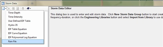
You can rename the rain file item or leave the default name. Once this is created, you will need to select the file being used. Click the ellipsis (“…”) button next to the item “Rain File” on the right and browse to the rain file being used. Change the items “Rain Data File Type” and “Rain Units” as needed. In the table on the right, enter a label, the return event (in years), the Station ID (which is likely in the rain file), and the time increment from the rain file.

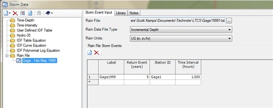
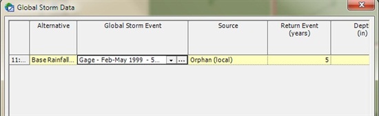
Click Close to return to the drawing. Next, select Components > Global Storm Event. In the pulldown for the column “Global Storm Event,” choose the storm you just created in the previous step.

Climatology Data

The previous steps are the same as applying any storm event to a CivilStorm or SewerGEMS model. The power of the Long Term Continuous Simulation is the ability to include other climatological data that can be used to get an accurate representation of the event. These include Temperature, Evaporation, Wind Speed, Snow Melt, and Areal Depletion. To add this data to the model, go to Components > SWMM Extensions > Climatology. These will be touch on briefly in the section below.

Temperature Data

The temperature data in this section is used to specify the temperature data used for snow melt computations. There are three selections. “No Data” is used when snow melt will not be simulated. “Climate File” is used when the data is in an external climate file. Choose this allows the user the import a DAT file with the data and specify the time that the data starts. “Time Series” refers to temperature variation over time. This selection opens a table in the Climatology dialog that allows the user to enter the time and temperature.

Note: The climate files that can be used for the “Climate File” option are DSI-3200 or DSI-3210 files available from the National Climatic Data Center, Canadian climate files available from Environment Canada, and user-prepared climate files where each line contains a recording station name, year, month, day, maximum temperature, and minimum temperature. The file can also optionally include evaporation rates and wind speed. If no data are available for any of these items on a given date, then an asterisk should be entered as its value. When a climate file has days with missing values, CivilStorm and SewerGEMS will use the value from the most recent previous day with a recorded value. User-prepared climate files must use the same units as the project being analyzed. For US units, temperature is in degrees F, evaporation is in inches/day, and wind speed is in miles/hour. For metric units, temperature is in degrees C, evaporation is in mm/day, and wind speed is in km/hour.

Evaporation Data

This section allows user to enter evaporation rates for the study area. There are a number of selections for this section. “No Evaporation” is used when evaporation will not be simulated. “Climate File” will reference the same DAT file used in the Temperature data tab. This cannot be used unless a climate file for temperature is specified. The user can enter values for the monthly pan coefficients in the table. “Monthly Evaporation” allows the user to enter the average evaporation rate for each month. “Constant Evaporation” means that the evaporation rate will remain the same throughout the simulation, independent of the time of year. “Time Series Evaporation” allows the user to enter the evaporation rate for a given time in the simulation.

Wind Speed Data

This section allows the user to input wind speeds. It is primarily used to calculate snow melt rates, as snow will melt faster at higher wind speeds. The units for wind speed are miles/hour (US Customary) and kilometers/hour (System International). “Climate File” refers to the wind speed data in the same climate file used for temperature and evaporation data. “Monthly Averages” allows the user to enter the average wind speed for a given month.

Snow Melt Data

This section allows the user to enter climatic variables for their study area. Default values are included, which can be adjusted for the area. “Dividing Temperature Between Snow and Rain” is simply the temperature where the precipitation from the rain file is assumed to snow instead of rain. “ATI Weight” refers to the Antecedent Temperature Index, which reflects the degree of heat transfer within a snow pack during non-melt periods is affected by prior air temperatures. Small values are used for deeper snow packs, which result in reduced rates of heat transfer. “Negative Melt Ratio” is the ratio of the heat transfer coefficient of the snow pack during non-melt conditions to the coefficient during melting conditions. “Elevation Above MSL” is the elevation of the area above sea level. “Latitude” is the latitude of the study area. “Longitude Correction” is a correction between true solar time and standard clock time.

Areal Depletion Data

Areal depletion refers to the tendency for a snow pack to melt unevenly over a surface. This tab allows the user to specify points for an areal depletion curve for both pervious and impervious surfaces.

Other Factors in LTCS

As mentioned above, LTCS can utilize a number of different inputs and parameters to running the simulation. These additional factors include aquifers, snow pack, infiltration, and groundwater.

Snow Pack

This is accessed by going to Analysis > SWMM Extensions > Snow Pack. These objects contain parameters that characterize the buildup, removal, and melting of snow over the follow sub-areas of a catchment: Plowable, Impervious, and Pervious. Each of these sub-areas have the same parameters, as defined in the Help documentation. This section also defines the Snow Removal parameters in a separate tab.

To create a new Snow Pack item, click the New icon. This will make the property fields editable and allow the user to go to the Snow Removal tab. To apply this to a catchment, open the catchment properties. Find the attribute “Has Snow Pack?” and set this to True. The Snow Pack created in this SWMM Extension can then be included.

Aquifers

This is accessed by going to Analysis > SWMM Extensions > Aquifers. Aquifers are sub-surface groundwater areas used to model vertical movement of water infiltrating from catchments. They also permit infiltration from groundwater into the system or exfiltration of surface water.

To create a new Aquifer, click the New icon and enter the required data. Definitions of these can be found in the Help documentation. To include this in the simulation, open the catchment properties and set the item “Apply Groundwater” to True. You will then be able to select the Aquifer created in this SWMM Extension.

Groundwater

Groundwater data are used to calculate the groundwater exchange between the aquifer and the node in the drainage system. A catchment contains the groundwater data and the user can view or edit the groundwater data in the catchment property grid. After setting the attribute “Apply Groundwater” to True, the groundwater parameters are opened.

The groundwater flow formula is described as:

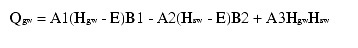
The coefficients and exponents in the catchment properties related to groundwater will be applied to this equation to calculate the flow of groundwater in the system.

Infiltration

Infiltration of rainfall from the pervious area of a catchment into unsaturated upper soil zone can be described using 3 different models: Horton, Green-Ampt, and SCS Curve Number. To successfully run SWMM5 engine, all catchments must use the same infiltration method. This can be assigned in the Calculation Options when using the Explicit (SWMM) engine. You can also assign it in the catchment properties.

Calculation Options

Once the data is inputted, it is time to compute the model. To make sure that everything runs correctly, you will want to make some adjustments to the calculation options (Analysis > Calculation Options).

First, LTCS works best with the SWMM engine. To change this, find Engine Type and change this to “Explicit (SWMM 5)”. Next make sure that the Simulation Start Date and Simulation Start Time match up with the date and time in the rain file used as the storm for the simulation. You will also need to set the end time. The easiest way to assure that this is correct is to change the field Duration Type to “End Date \ End Time” and enter the End Date and End Time that corresponds with the rain file.

Other possible calculation options that are used include “Start Sweeping On” and “End Sweeping On” which are included when street sweeping activities are expected to impact the simulation. “Catchment Results Type,” “Nodes Results Type,” and “Links Results Type” specify the degree of results generated for the different element types. This can include all results, no results, or results for a given selection set of elements.

It is also possible to save and use Rainfall Files, Runoff Files, and RDII Files. For more information, see the following link:

LTCS also supports Hot Start files. Hot start files are binary files created by the SWMM engine that contain hydraulic and water quality variables for the drainage system at the end of a run. The hot start file saved after a run can be used to define the initial conditions for a subsequent run.

Hot start files can be used to avoid the initial numerical instabilities that sometimes occur. For this purpose they are typically generated by imposing a constant set of base flows (for a natural channel network) or set of dry weather sanitary flows (for a sewer network) over some startup period of time. The resulting hot start file from this run is then used to initialize a subsequent run where the inflows of real interest are imposed.

It is also possible to both use and save a hot start file in a single run, starting off the run with one file and saving the ending results either to the same or to another file. The resulting file can then serve as the initial conditions for a subsequent run if need be. This technique can be used to divide up extremely long continuous simulations into more manageable pieces.

When this field is set to True a hot start file will be generated from the end results of the run. More information on this can be found in the Help documentation.

Viewing Results

After computing the model, you can view results just as you can with any other model file. This includes graphs, profiles, and viewing results in the properties or element FlexTables.

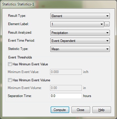
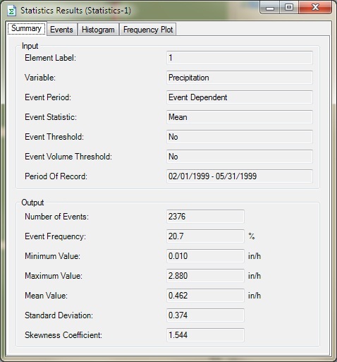
Another useful tool is the Statistics dialog (Analysis > More > Statistics). LTCS results generate lot of output data, in that case statistics tool is helpful to look at statistical results, here you can save multiple analyses in Statistics manager just like creating multiple scenarios in one model.

With this tool you can specify following,

Select an element from previous selections or choose the element from model
The result field to be analyzed e.g. precipitation, runoff losses etc. this is the result variable to be analyzed.
Event time period - allows you to choose the length of the time period that defines an event. Which can be dependent on the event / daily / monthly / yearly i.e. annual likewise. In the Event-Dependent case, the event period depends on the number of consecutive reporting periods where the simulation results are above the threshold values defined below in the Event Thresholds section of the dialog. That is, how much rain constitutes an event and what period of time between non-zero rain constitutes a separate event.
And the statistic type - to define the type of statistical analysis to perform. These include Mean, Peak, Total, Duration and Inter-event time.
You can also set minimum and maximum event thresholds, these fields allow you to refine the criteria that delineates events.
Separation time - this is the minimum number of hours (time can be in days, hours, minutes) that must occur between the end of one event and the start of the next event. Generally events with fewer hours are combined together for the analysis.

When you click the Compute button, you get a series of results depending on the statistic type you used. It reports the events in the order they happened in events tab, histogram will show a plot of occurrence frequency versus event magnitude. Frequency plot is graph of exceedance frequency vs. event dependent mean values of selected variable, which shows % frequency of events which certain mean values of given variables.

Performance

When computing a long term simulation, the amount of time it takes to complete the calculation (the performance) can be a factor. CivilStorm and SewerGEMS currently do not have the ability to utilize your GPU (such as CUDA cores), but there are several features available to improve performance.

1) Ensure that you have the Explicit (SWMM) solver selected as the active numerical solver in your calculation options. This will be much faster for a Long Term Simulation.

2) In the calculation options, choose the appropriate granularity for timesteps. This includes the Output increment (how often the results will be reported), the Routing step (how often the results are calculated - the larger the value, the faster the performance, but with reduced accuracy), and the "Results Type" fields (where you can choose a selection set to report results for only a subset of elements if desired).

3) In the calculation options, consider setting the "Skip Steady State Periods?" option to true. If you have long dry periods between rain events in a long term simulation, this can help speed up performance.

4) In the calculation options, consider adjusting the "number of threads" option. This can use multiple CPU cores - the parallel calculations can speed up performance.

5) Address all data entry issues that could cause excessive numerical trials during calculation. Check your User Notification list for specific issues, and review model data entry (for example check profiles), as mistakes could potentially cause the numerical solver to struggle to solve. Where possible, simplify any overly complex sections of the model network which could cause the solver to struggle.

6) Assess your computer CPU and memory specifications and upgrade if desired. The faster the CPU clock speed (and the newer the architecture generation), the faster the performance. For larger models that may take up a large amount of memory, consider the amount of physical memory (RAM) on the system and upgrade if needed.

7) Ensure that the Windows Temp folder are located on a high speed Solid State Drive (SSD - as opposed to traditional spinning hard drive, HDD). This will improve the performance of the model as it saves results to the temporary folder. Storing the model file itself on a SSD will also improve performance while opening and working with the model, and the initial data loading part of the calculation process.

8) Perform the "Compact Database" operation on your model - this usually would only improve performance when opening and working with the model, though.