| Product(s): |
WaterGEMS, WaterCAD, SewerGEMS, SewerCAD |
| Version(s): |
V8i, CONNECT Edition |
| Area: |
Modeling |
|
Original Authors : Scott Kampa, Jesse Dringoli, Tom Walski |
Background
If you are modeling only a portion of a larger system, you may have a need to model the hydraulics of the connection to that existing system. This can happen for example when modeling a proposed expansion (such as a new subdivision, industrial park, school, shopping mall, etc.). Frequently, the engineer will not have complete information on the system to which they are connecting, and must decide on an appropriate approach for modeling this connection.
The most reliable method for representing the existing system is to include a least a skeletonized (simplified) representation of the significant system components that affect the project area. Typically, this representation would include tanks, pumps, control valves, and significant demands in the same pressure zone. This necessary information can usually be obtained through water utility mapping and modeling personnel.
Another method for approximating a connection to an existing system is to represent the connection point as a constant head elevation using a reservoir element. This is a very simplified approach, and usually a very unreliable one, since it doesn’t account for the drop in hydraulic grade that will likely occur as inflow increases. This may depend on the type of system you are connecting to. For example if you are connecting to large diameter pipes, then the hydraulic grade at the connection point may not drop much as flow enters your proposed system, in which case the reservoir approach may be acceptable. However if you are connecting to small diameter pipes (such as 6 or 8 inch diameter), the hydraulic grade is likely to drop significantly as flow increases, especially during a fire. In this case the reservoir approach may not be acceptable.
Note: see Sewer Applications if you are modeling a connection to an existing downstream sewer force main (pressure network).
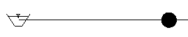
The reliability of the method described in this article lies somewhere between the two just described. It consists of representing the connection to the existing system as a reservoir and a fictitious pump with a 3-point characteristic curve based on static and residual pressure obtained during a two-hydrant flow test near the connection point. The fictitious pump will simulate the pressure drops and the available flow from the existing water system.
Unlike the first approach described, this third method does not allow the engineer to capture the changes at the connection point due to, for instance, fluctuating tank levels and pump status changes in the supply system. However, it does allow for consideration of change in head due to variation in the demand at the connection point. When combined with a good general understanding of how the larger system performs under a range of conditions and knowledge of system conditions (e.g., tank and pump status) at the time flow tests were performed, it can be an acceptable approach in many instances. It is usually most appropriate for “fill in” development where most of the customers and infrastructure are already in place as opposed to large expanses of undeveloped land at the fringe of an existing system. If model results obtained using this method are near the borderline of being unacceptable, the engineer should revert to the more rigorous first approach.
NOTE: This method is only an approximation, so the results will not be as accurate as if you modeled the system back the actual source. It is also important to note that you cannot model multiple connections to an existing system. The results in such a case could be skewed and will not be viable.
In order to simulate the range of pressures at the connection point for a range of flows, you must first obtain two-hydrant flow test data. To represent zero flow, you'll need the static pressure. To represent the highest flow possible through the connection, you'll need the residual pressure and flow. To convert the pressures to hydraulic grade, you will need to know the exact elevation of the residual pressure gage. This data is obtained from field tests.
For more information on how to perform a field hydrant test, you may refer to section 5.2 of Advanced Water Distribution Modeling and Management.
NOTE: The flows you obtain from the hydrant test must be in actual flow units such as gallons per minute, not pitot gage pressures. Equation 5.1 in Advanced Water Distribution Modeling and Management provides a conversion.
Steps to Accomplish
The reservoir element simulates the supply of water from the existing system. The Elevation of the reservoir should be equal to or slightly higher than the elevation at the connection point as explained in this article. The pump and the pump curve will simulate the pressure drops and the available flow from the existing water system. The points for the pump curve are generated using a mathematical formula (given below), and data from a hydrant flow test. The pipe between the fictitious reservoir and pump should be smooth, short and wide so as not to contribute headloss. For example, a Roughness of 140, length of 1 foot, and diameter of 48 inches are appropriate numbers. Please note that it is ALWAYS best to model the entire system back to the source as mentioned further above. The reservoir+pump method is only an approximation, and may not properly represent the water system under all flow conditions.
Qr = Qf * [(Hr/Hf)^.54]
where:
Qr = Flow available at the desired fire flow residual pressure
Qf = Flow during test
Hr = Pressure drop to desired residual pressure (Static Pressure minus Chosen Design Pressure)
Hf = Pressure drop during fire flow test (Static Pressure minus Residual Pressure)
Determining the Three-Point Pump Curve
Below is an example of how the three-point pump curve is developed. This will use the flow test results from your system, but the steps below will be same once you have that data.
1. The first point is generated by measuring the static pressure at the hydrant when the flow (Q) is equal to zero.
Q = 0 gpm
H = 90psi or 207.9 feet of head (90 * 2.31)
(2.31 is the conversion factor used to convert psi to feet of head).
2. The engineer chooses a pressure for the second point, and the flow is calculated using the Formula below. The value for Q should lie somewhere between the data collected from the test.
Q = ?
H = 55 psi or 127.05 feet (55 * 2.31) (chosen value)
Formula:
Qr = Qf * (Hr/Hf)^.54
Qr = 800 * [((90 - 55) / (90 - 22))^.54]
Qr = 800 * [(35 / 68)^.54]
Qr = 800 * [.514^.54]
Qr = 800 * .69
Qr = 558
Therefore, Q = 558 gpm
3. The third point is generated by measuring the flow (Q) and the residual pressure of the hydrant.
Q = 800 gpm
H = 22 psi or 50.82 ft. of head (22 * 2.31)
Pump curve values for this example:
Head (ft.) Discharge (gpm)
207.9 0
127.05 558
50.82 800
Setting up the Model
To set up the model, you will enter the pump curve just developed, lay out the model elements, and enter their attributes within your project area.
1. Open your model in WaterCAD/WaterGEMS (or open the existing model if you have already laid out the elements for the new system) and go to Components > Pump Definitions.
2. In the Pump Definitions Manager, click the "New" button and name your pump definition appropriately (such as "Connection").
3. Keep the default Pump Definition Type of "Standard (3 point)" and enter your data in the table:
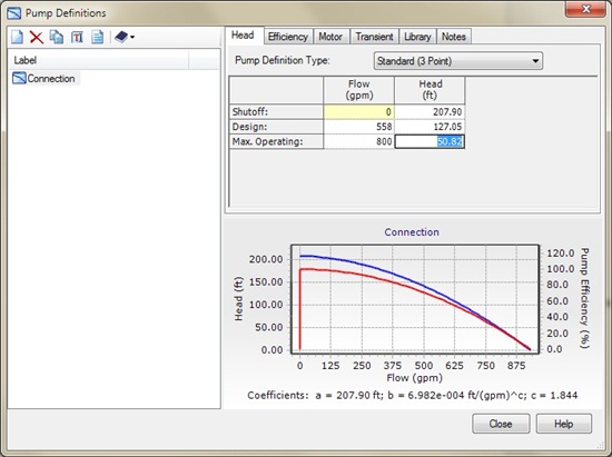
4. Click the "Close" button to accept the curve, which we will use further below.
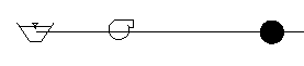
5. Now lay out the elements in the model (if this is not already done). You will need a reservoir and pump, which represents the connection to an existing system.
6. To adjust the attributes of these elements, first open the properties of the reservoir node and set the "Elevation" attribute to the elevation of the pressure gauge used at the hydrant, since this is the point from which the hydrant pressures (the source of the fictitious pump curve) were measured. To explain further: the head points on the fictitious pump curve are calculated based on the pressure as measured from the hydrant elevation. They represent the head available at the connection point, above the reference point where the pressure was measured from (elevation of the pressure gauge at the hydrant). In order for the fictitious pump to produce the correct pressure/hydraulic grade in the downstream new system, it needs to add those heads to the hydrant elevation. This is why you enter the pressure gauge/hydrant elevation as the elevation of the upstream reservoir element, since a reservoir acts as a boundary hydraulic grade; it sets the hydraulic grade and then the pump adds head to it to achieve the downstream pressure.
Note that the pipe connecting the reservoir to the pump which be such that the hydraulic impact is negligible. For example, a Roughness of 140, length of 1 foot, and diameter of 48 inches are appropriate values.
7. Open the properties of the junction element immediately downstream of the pump. This point represents where the proposed system begins, so enter the physical elevation of the connection point.
8. Open the properties of the pump element and select the pump definition you created in step 3 from the "Pump Definition" dropdown. Set the "elevation" slightly below the elevation of the reservoir (slightly below the elevation of the pressure gauge, where the pressure was measured from). The elevation of the pump is of little importance since it just determines the calculated pressure as reported from the pump itself and does not influence the downstream pressure (since the pump is adding head to the upstream boundary condition to achieve the downstream pressure). However if you simply set the pump elevation equal to the reservoir elevation, any slight headloss in the pipe between the pump and the reservoir will result in a hydraulic grade slightly below the pump elevation and you'll see a user notification about negative pressure. So by setting the elevation slightly below the reservoir elevation, you'll avoid the negative pressure notifications.
9. Make sure the rest of the system is set of correctly and compute the model. The pump should react according to the proposed system demands to provide an approximation of head at the connection point.
Assumptions and Limitations
This approach is an approximation, the accuracy of which depends on a number of factors.
It is better to model all the way back to the source, at least by obtaining skeletonized data on the existing system. The skeletal model must begin at the real water source(s), such as the pump or tank, which will serve as the primary water source(s) for the new extension pipes. It should be calibrated using the results of fire hydrant flow tests, especially the tests conducted near the location where the new extension will tie in. You may need to call the municipality to obtain basic information on the existing system.
Using the pump approximation method can present problems because this approximation of the existing system only accounts for the exact boundary conditions and demands that existed at the time that the test was run (for example, the afternoon on an average day with one pump on at the source). Basically, the simulated connection is only valid for the conditions present during the hydrant tests. Therefore, determining the effect of changing any of the demands or boundary conditions is difficult. An extended period simulation (EPS) that is performed using the pump approximation method will be less accurate and may not provide reliable data regarding projected changes in consumption. The pump approximation approach only works well if the existing system is fairly built-out near the connection point and the demand and operation conditions are expected to remain essentially the same in the long run. The hydrant flow test is useful for predicting changes in pressure when downstream demands change, but not for evaluating other types of system changes such as the addition of new pipes, or operational alternatives such as fire pumps starting up.
Modeling more than one connection between the proposed expansion and the existing system may not be a valid approach.
Some reasons for this are, first, the hydrant tests were most likely done at different times, yet the model will allow water to be taken from both sources at the same time. This is not accurate because in reality, both sources will not be able to provide the full observed residual pressure when open at the same time. In other words, if hydrants or connections were really opened at both connection points simultaneously, the combined flow would result in a much reduced residual pressure at both locations versus what was observed during the independent tests. Secondly, in some cases, depending on the hydraulic grades, it may be possible for flow to enter at one connection point and exit at another. However, the pump element only allows water in the forward direction, so the pump approximation method would not work in this case (and may provide a message about one of the pumps not being able to deliver head). The situation is too complex to model using a method other that a skeletonized representation of the larger system.
However, if you are modeling a system where the upstream system will not experience a significant change in pressure as a result of multiple connections flowing at the same time, or if there are separate, disconnected systems upstream of each connection point, modeling multiple connection point may be fine.
As the size of the modeled system increases and the number of connection points increases, it may not be reasonable to separate the development site from the rest of the system and achieve accurate results. The interactions may be too complex. One suggestion in this case is to get together with the City water distribution engineers and discuss how to model this. Ideally you would get a copy of the City model (at least the pressure zone of interest) and build your model on top of it. Or you can get their distribution maps and build very simple skeletal model of the system. You need to model back to some real boundary condition.
One, somewhat far fetched, test might be to run (assuming you have 6 connection points) 6 simultaneous flow tests. You couldn't run all the hydrants wide open (unless you have a very strong system) without lowering the pressure too much. So, if your demand is 1800 gpm for example, you could run 300 gpm at each flowed hydrant. This isn't as good as running a model of the full pressure zone but at least it gives you an idea of what a 1800 gpm demand will do to the City system.
Attempting to compute the 'static' (no demand) conditions of the new model with the pump approximation in place will most likely result in an unbalanced simulation.
In this case, you may need to model the connection simply as a reservoir with an elevation equal to the pressure gauge elevation and static pressure head (i.e., the static HGL), or simply manually compute the static pressure at each node by taking the difference between the static HGL and the node physical elevation.
Sewer Applications
Connection to un-modeled downstream system
For a sewer force main (pressure sewer system) in SewerGEMS or SewerCAD, you may have a need to model a pump for a specific area and do not have the full downstream model. In this case you will need to approximate the hydraulics of the connection point (manifold) to the downstream system. This can be done using an outfall node element (for SewerCAD and SewerGEMS, or a reservoir if modeling this in WaterCAD or WaterGEMS) to establish the boundary hydraulic grade that the upstream pump will be pumping against. Set the elevation of the outfall to the pipe elevation, set the bounndary type to user defined tailwater, and set the user defined tailwater equal to the hydraulic grade in the existing force main (pressure head plus elevation). Or if using WaterCAD or WaterGEMS to model this, set the reservoir elevation to the hydraulic grade that you will be assuming at the connection point.
However, the elevation that you choose will not always be accurate for all times. The pressure that you are tying into may depend on how many other pumps are running in the un-modeled system, and will also be influenced by the additional flow that you are adding to that system. Meaning, you may measure a pressure of 50 psi for example at the connection point right now, but when your pump is tying in and adding additional flow, that increases the downstream headloss, which will cause the pumps in the existing system to add more head, which will increase the pressure at the connection point. You could use a rating curve as the outfall boundary type, but the rating curve would need to be determined.
As seen further above, in a water distribution system application hydrant flow tests can be used to determine how the pressure changes as the flow changes, but in a sewer application you likely cannot simply inject a range of flow near the tie-in point to determine this (and then model it as an outfall with elevation-flow rating table). So, a conservative assumption may need to be made for the tie-in pressure (outfall elevation), perhaps based on any data that you happen to know about the system. Ideally you would be able to access a hydraulic model of the entire system, or at least a skeletonized version.
Connection to un-modeled upstream system
In some cases you may need to start your model at a connection point. Meaning, there is an upstream portion of the network that is not being modeled, and the model is cut-off at the connection point. In this case, you may have information describing the flow through that point in the network in the real system or a larger version of the model.
In these cases, you can start the network at that point with either a cross section element (for a channel) or a manhole (for an underground pipe). In the properties of the cross section or manhole, open the inflow collection and specify a hydrograph inflow. You can paste in the values if you have them from an external application. If you have the flow results from another model (such as a larger version that includes the upstream elements), graph the flow in that model, click the data tab, then copy the time/flow columns from there. When pasting into the inflow hydrograph (in the model where you are not modeling the upstream system), make sure the time and flow units match up, then after pasting, check the first and last row to make sure a duplicate 0,0 entry was not added.
so that the upstream-most starting point of the network is